Free Matlab alternative

GNU Octave is a free, scientific programming language. It offers a rich mathematical apparatus, concise syntax, and has built-in visualization tools [1]. The whole package is really handy. It has a graphical user interface (GUI) and command-line interface versions. It feels like a standard Integrated Development Environment (IDE) for Java or Python.

Octave can be used for solving various mathematical problems, building simulations, or working on data science projects. If you’re familiar with Matlab [2], or you’re looking for a quick way of prototyping your science-related ideas, you should definitely try Octave. Let’s go through practical examples that will help you to start your journey with this tool.

Installation

On Debian operating systems (e.g. Ubuntu) you can install Octave by using the built-in package manager:

If you’ll be prompted about missing packages check here [3] for the command with full a list of needed packages for your version of the operating system. For ubuntu 20.4 it looks like this:

If you’re using Windows simply download the installer executable file or a zip file and unpack it. Current version 5.2, and instructions for macOS and BSD systems, are available here [4].

GUI guide

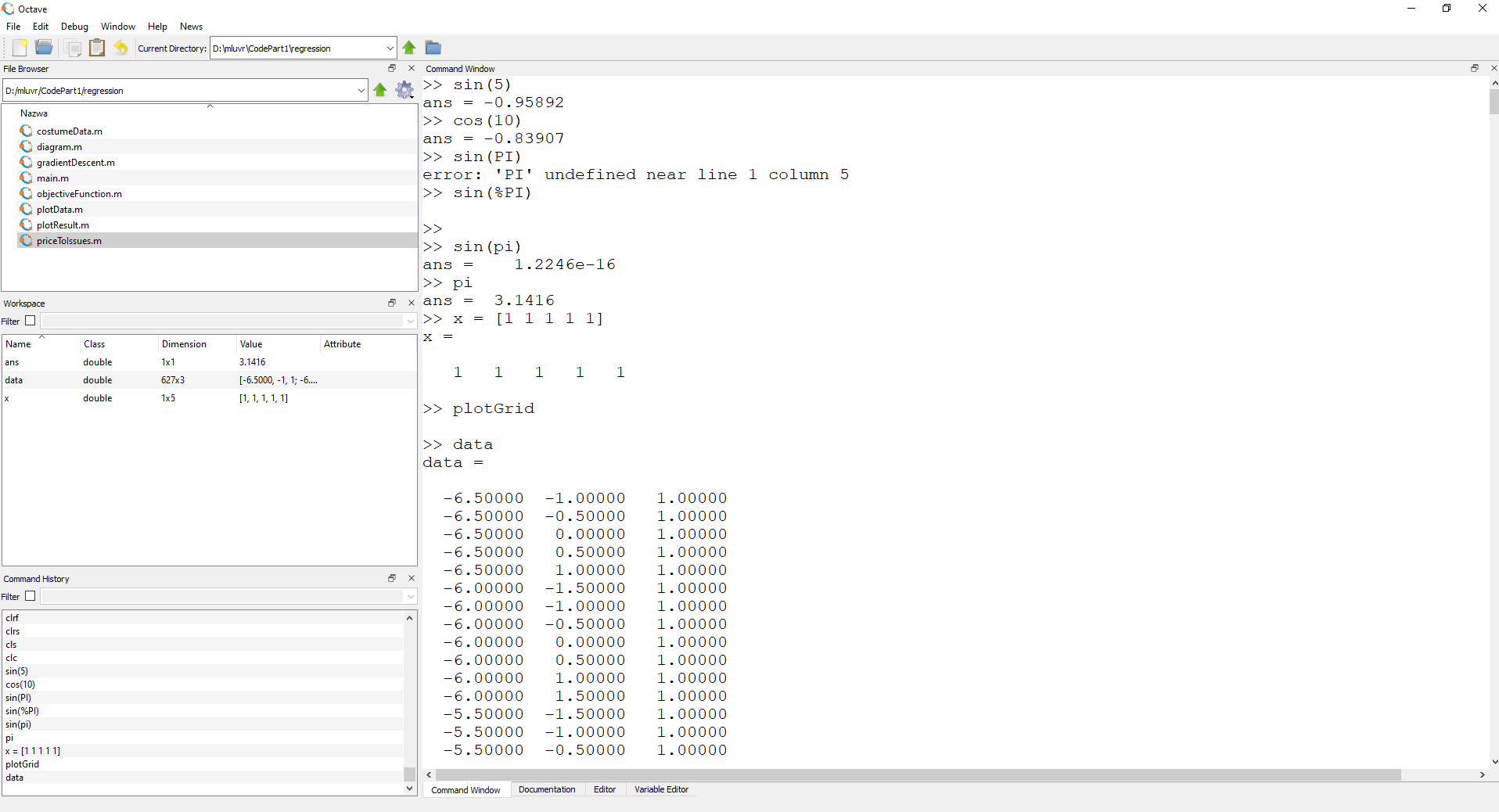
Octave GUI consists of 4 main parts. The most important one is the panel that covers the biggest area on the right. By default, it is a Command Window. Here you can type any Octave commands in interactive mode and they are immediately executed, showing the result.

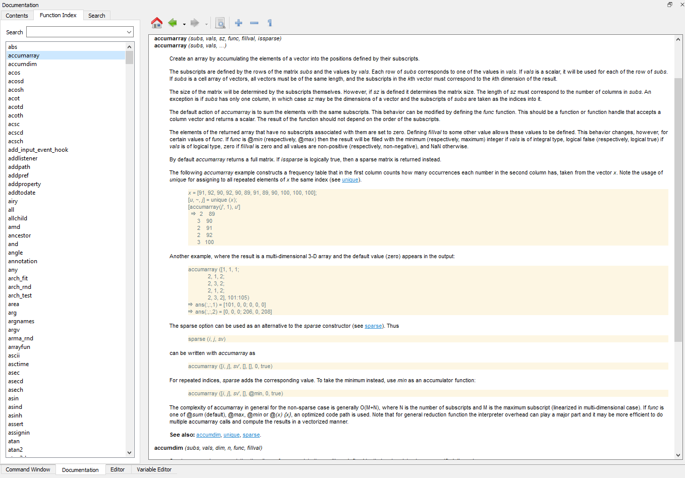
At the bottom of the Command Window, you can find another 3 tabs. The second one is Documentation. It’s a very handy, offline version of the whole Octave docs. It is divided by themed sections where you can read about topics like Data Types or Statements. It also contains a separate functions index with examples:

The last two tabs under the main area on the right are Editor and Variable Editor. The editor tab is simply a text editor where you type your Octave code. It has a syntax completion feature, but in general, is quite minimalistic. In Variable Editor, you can choose a variable and change its values. It is useful while dealing with multidimensional variables, so you don’t get confused when you need to edit them by hand. From my experience, it’s quite rarely used functionality.

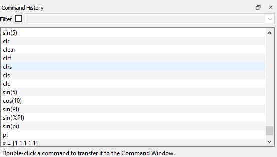
On the left part of the main window, there are 3 panels. At the top, there is a File Browser where you choose your project directory and can manipulate its files. Below you’ll find a Workspace that contains all active variables as well as their short descriptions (type, dimension, values, attributes). The last panel contains Commands History. It allows you to search for and filter the commands you used in the past:

Working with data

Data and variables are core parts of any computer program. Take a look at how to define different types of variables and load files in Octave.

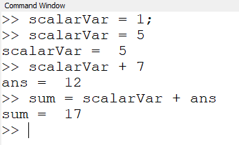
In the screenshot, you can see that defining variables is pretty intuitive. You need to provide a variable name, use assign operator “=” and type a value you want to put under the variable. You can use scalar values like integer numbers, floating-point numbers, text (defined in quotes like “I’m a sample text”). If you just put a value without a name, Octave creates ans variable and keeps there the last value you typed directly in the command window. You can use ans as any other variable.

If you looked at the screenshot carefully, you noticed a trick. When you end your line with a semicolon “;” the command doesn’t print any output. However, commands without a semicolon at the end print the result to the console.

Defining vectors

A vector is a variable that consists of multiple values. You can think of it as of array of elements. To define a vector in Octave you need to provide a vector name and its values separated by space. All statement should be enclosed with square brackets:

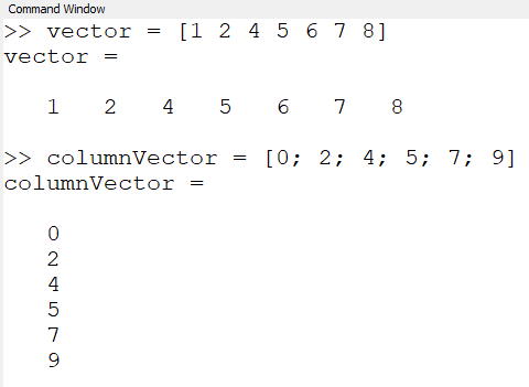
To define a column vector you should separate vector values using a semicolon.

Defining matrices

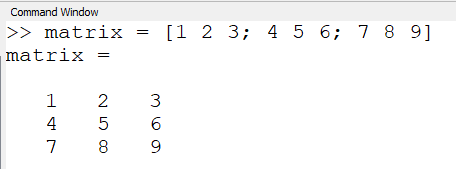
Matrix definitions are as straightforward as vector ones. The main rules are:

1. Separate matrix row values with spaces.
2. Separate matrix columns with semicolons.

Take a look at the picture:

Functions useful while defining variables

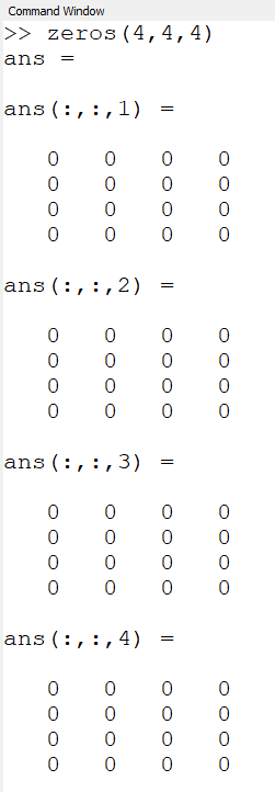
If you want to generate a variable consisting of zeros or ones there are two convenient functions you can use. zeros(m,n,k,..) generates variable full of zeros and m,n,k are integers defining the sizes of dimensions. By analogy you can use ones(m,n,k,…) to get a variable filled with ones:

Another useful way of generating values is generating vectors using given discrete steps. Let’s assume you need a vector that goes from zero to 10 with a step equal to 0.5. In Octave you can define it like this:

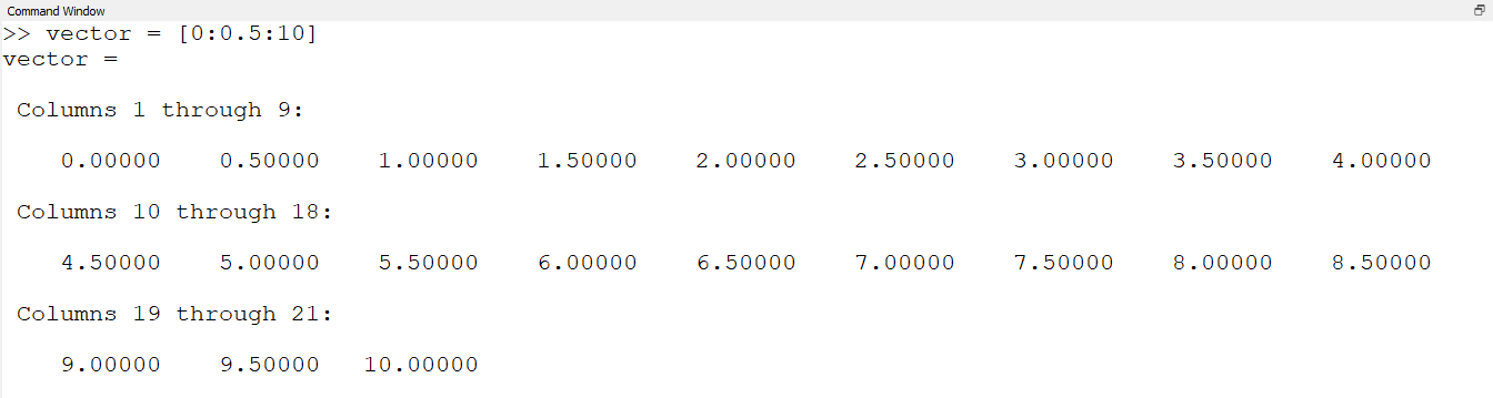
All you need to do is to start with the initial value, step value, and the last value of the vector. These three values should be separated with a colon. In our example vector has 21 elements.

Accessing elements

One of the most important things to remember while accessing variables is that Octave starts indexing from 1, not from 0 as most of us are used to. To get the particular element you need to specify its indices inside parenthesis:

Loading data

The easiest way to load the data is to use load(filename.m) function. It expects to have a file with comma-delimited values and columns. Take a look at the example:

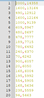
Having such a file, let’s call it myData.m, you simply choose a variable to assign the data and call load function like this:

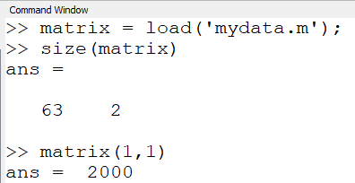
In the picture, you can see that we loaded a matrix variable which has 63 rows, 2 values each. To check the variable size the size(variable) function is used. After loading we check the first element of the first row which is equal to 2000.

Octave also supports more advanced loading functionalities like binary files or defining the delimiter inside the file. To find out more check the load function description in the documentation.

Basic linear algebra operations

The most powerful part of Octave is a built-in mathematical apparatus. The straightforward and handy syntax makes it even better.

Adding and subtracting matrices

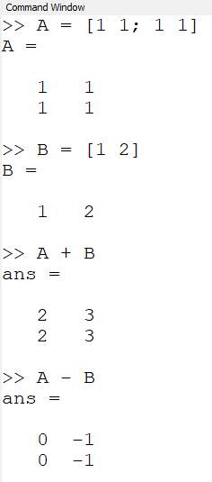
To add or subtract matrices you need to use “+” or “-” minus operator. When you add two matrices of the same sizes the operation will be done using values from corresponding cells (e.g. value from the first row and first column from matrix A plus value from the first row and first column from matrix B).

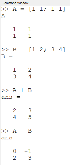
However, you need to be careful. It is also possible to add or subtract a vector. To make it clear let’s look at a couple of different examples:

Matrix multiplication

Let’s recall the prerequisite needed to multiply matrices.

To multiply matrix A of size m x n by matrix B, the number of rows in matrix B must be equal to the number of columns in matrix A. Assuming that matrix B has size n x k, the result of the multiplication is the matrix C of size m x k. To multiply matrices use the “*” operator.

Let’s take a look at the example:

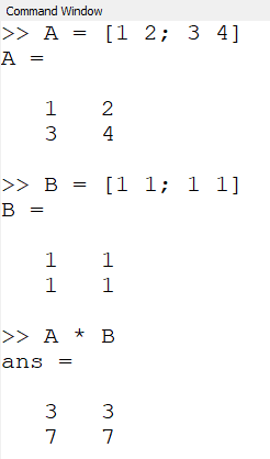
Why we get such a result? Check how each matrix cell is calculated according to matrix multiplication rules:

We can apply the same rule to vectors, as they are a special case of matrices (size of 1 x n, or n x 1 in case of column vectors). We’ll get a single value if we multiple vectors of the following sizes:

To visualize this case let’s define vector A and a column vector B and multiply them:

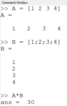
Both vectors consist of 1, 2, 3, 4. Multiplying them is equal to multiplying first elements from A and B and adding the result of multiplication of their second elements and so on until we reach all of the elements. It means we get:

Scalar matrix multiplication

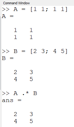
Sometimes you need to multiply corresponding elements of matrices. Of course, it’s not the matrix multiplication according to linear algebra definition, so you can’t use the “*” operator. Instead, Octave has an additional dot “.” operator that goes before the multiplication operator. Let’s see what happens when you use it:

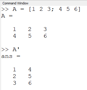
Matrix transposition

To transpose a matrix, it means that we change the rows to the columns and the columns to the rows. As a result, the size of the matrix changes according to the following formula:

In Octave you can transpose a matrix by using the “ ‘ “ operator:

Solving a linear equations system

Finally, let’s solve a simple linear equations system:

Such a system can be represented by two matrices that map coefficients before variables. The first one represents the left side of the system:

And the right side looks like this:

The whole system is represented using the following formula where matrix x consists of variables x and y:

To solve it we could invert matrix A and multiply it by matrix b. In Octave, it is equivalent to using left side division operator “\” [5]. As a result x = A \ b:

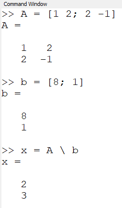
Finally, we got that variable x equals to 2 and variable y equals to 3. That’s the correct answer, great!

Visualization tools

We know that image is worth thousands of words and it can help to understand the problem we try to solve. Fortunately plotting is also a built-in functionality of Octave.

Plotting points

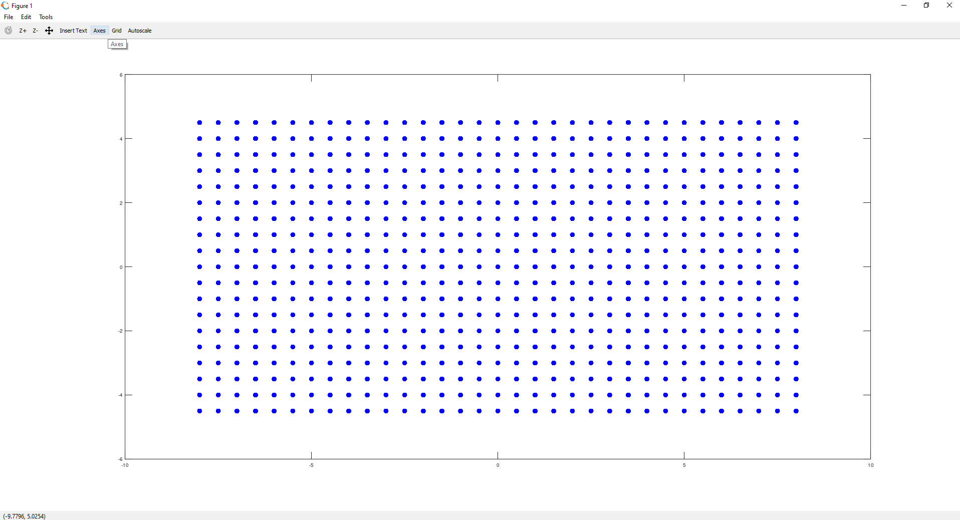
To draw a 2D data point you can use plot function. It takes x and y coordinates of your points as arguments and additional style-related parameters.

Let’s assume you have a file in which every line contains a point. The code below loads the file into data variable, extracts the x and y coordinates of each point (using the “:” operator), and plot blue points (“b.”) points of size 30 (“markersize” parameter):

As a result, we get a grid of points:

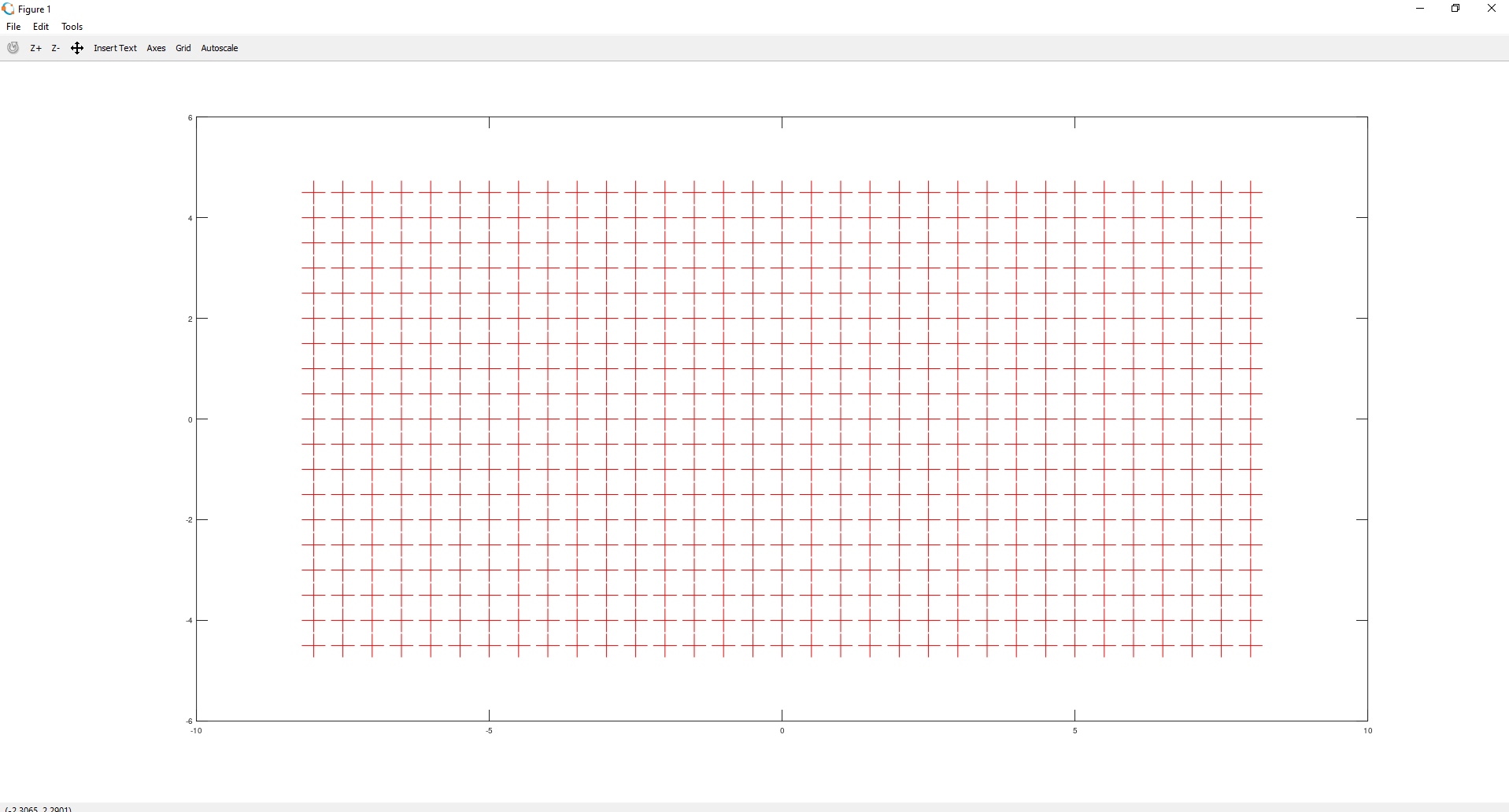
To change colors and style you can try different letters, e.g. g for green, r for red, and for points style characters like “+” or “*”. For example “plot(x, y, ‘r+’, ‘markersize’, 30);” looks like this:

Plotting functions

You can use the same plot method to draw a function graph. First of all, you need to prepare your vector of discrete coordinates and then a vector of function values for each of the coordinates. What’s important these vectors should have equal sizes.

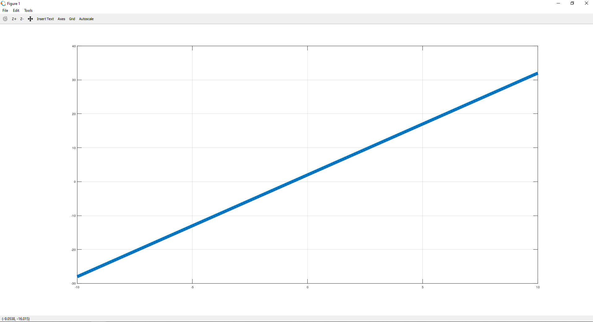
As an example let’s draw a plot of the following function:

Take a look at the code snippet:

In the first line, vector x starts from -10 and is filled until values reach 10 (with the step equal to 0.1). So it contains -10, -9.9, -9,8 … 10. Then vector y contains values of the function for each x coordinate. Finally, we plot our function and set its line width to 10:

More fancy functions

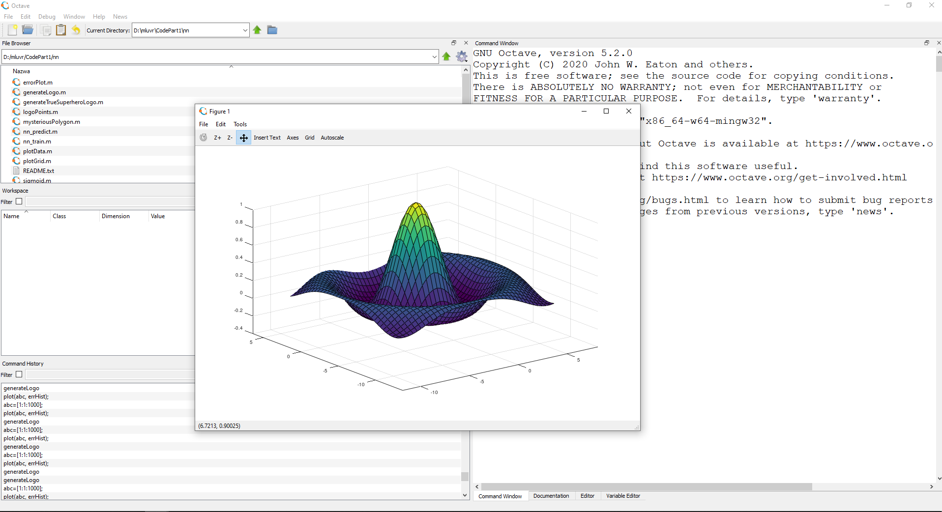
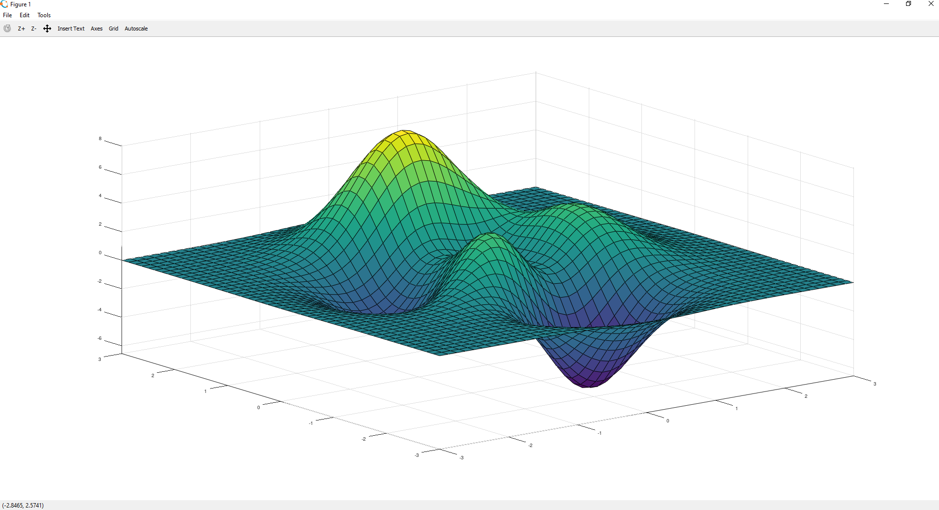
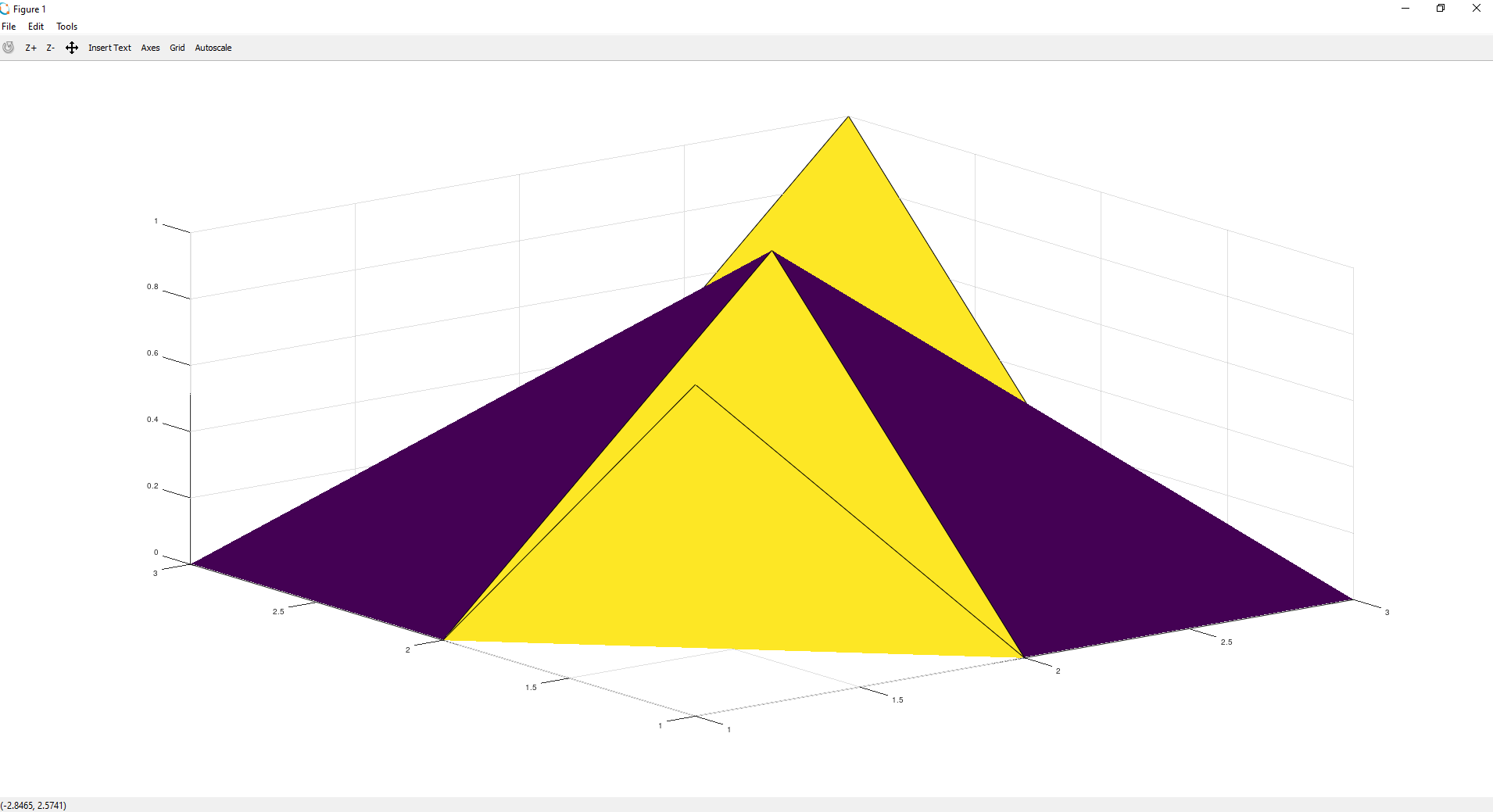
Of course, it’s possible to draw more complex functions. Octave provides really good documentation, so I encourage you to check and play with plot3, meshgrid, surf, sombrero functions. It’s a good exercise.

For some of the functions mentioned above Octave also provides some test plot function, you can quickly see the result just by calling them without any parameters. Here are some examples:

Useful trick

For the last point of this crash course, I’ll share functionality which is really useful while filtering your data. You can use it on the vector or matrix of predictions from your Machine Learning classifier and decide about labels of given objects. Another example is applying a given threshold to your data or removing and extracting anomalies.

Let’s assume we have a predictions vector containing 0 and 1 as labels for different objects. To find the indices of a given label you can use find function and define a condition as its parameter. To understand it better, let’s check the following example:

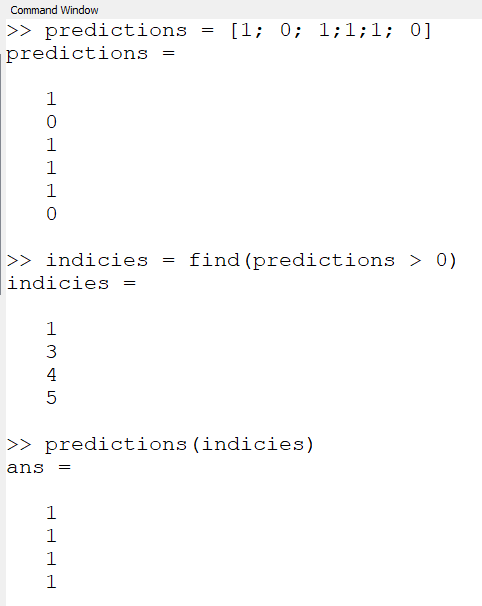
How does it work? The condition passed to find function is used to return all indices of elements that are greater than 0. Then we can use those indices to extract elements from the predictions vector. That’s it!

Summary

After completing this short tutorial you have the knowledge which should give you a kick start to the Octave environment. You know how to define and load data, how to perform operations on vectors and matrices, and how to visualize your work.

I encourage you to use Octave whenever you came up with an idea and you need a rich yet straightforward environment to prototype it, and your full-blown Python setup is out of the reach.

Bibliography:

1. https://www.gnu.org/software/octave/
2. https://en.wikipedia.org/wiki/MATLAB
3. https://wiki.octave.org/Octave_for_Debian_systems
4. https://www.gnu.org/software/octave/download.html
5. https://octave.org/doc/v4.0.1/Simple-Examples.html