## This sheet simulates a 'substrate depletion' regulatory network
var('k0 k00 k1 k11 k2 k22 k3 k33 k4 k44')
var('J1 J2 J3 J4')
var('X R S E t')
var('X0 R0 S0 E0')
## INITIAL CONDITIONS
X0 = 5 ## 1.5 5
R0 = 0.1 ## .2 2.1
S0 = 0.000 ##
t0 = 0.000 ##
## CONSTANTS
k0 = 1
k00 = 0.000 # 0.01
k1 = 1
k2 = 1
k3 = 1
k4 = 1
J3 = 0.05
J4 = 0.5
S = 0.2
## CALCULATION PARAMETERS
end_points = 100
stepsize = 0.1
steps = end_points/stepsize
dvar = [X,R]
ivar = t
ics = [t0,X0,R0]
## EQUATIONS
G(u,v,J,K) = (2*u*K)/(v-u+v*J+u*K+sqrt((v-u+v*J+u*K)^2-4*(v-u)*u*K))
E = G(k3*R,k4,J3,J4)
r1 = (diff(X,t) == k1*S-(k00+k0*E)*X)
r2 = (diff(R,t) == (k00+k0*E)*X-k2*R)
## NUMERICAL SOLUTION OF A SERIES OF DIFFERENTIAL EQUATIONS
des = [r1.rhs(), r2.rhs()]
sol = desolve_system_rk4(des,dvar,ics,ivar=t,end_points=end_points,step=stepsize)
#show(sol)
|
|
sols_1=[]
sols_2=[]
for i in range(steps):
sols_1.append([sol[i][0],sol[i][1]])
sols_2.append([sol[i][0],sol[i][2]])
################################################
#### Unnecessarily Fancy Plotting Stuff ####
################################################
## Create a plot object
a = plot([])
## Set the plot parameters
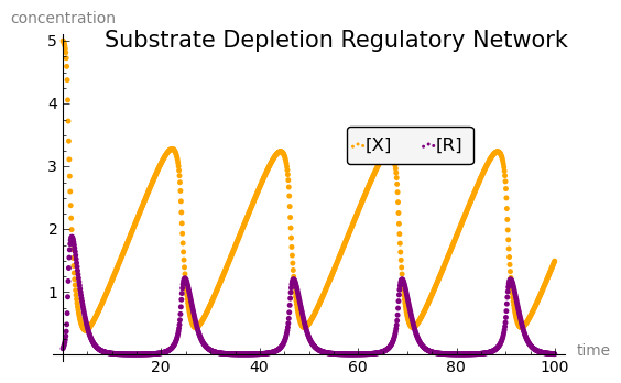
title = "Substrate Depletion Regulatory Network" ## Graph Title
xmin = 0 ## X minimum
xmax = end_points ## X maximum
ymin = 0 ## Y minimum
ymax = 5 ## Y maximum
## Add a title to the plot
a += text(title,(xmax/1.8,ymax),color='black',fontsize=15)
## Add the desired lines to the plot
a += list_plot(sols_1,color='orange',legend_label='[X]')
a += list_plot(sols_2,color='purple',legend_label='[R]')
## For more information on plots in general, evaluate 'plot?'
## For a list of legend options, evaluate 'a.set_legend_options?'
## For a list of Sage predefined colors, evaluate 'sorted(colors)'
a.set_axes_range(xmin,xmax,ymin,ymax)
a.axes_labels(['time','concentration'])
a.axes_label_color('grey')
a.set_legend_options(ncol=2,borderaxespad=5,back_color='whitesmoke',fancybox=true)
show(a)
|
sols_0 = []
## Grab a slice of steady-state oscillations for later use
for i in range(steps*0.8,steps):
sols_0.append([sols_1[i][1],sols_2[i][1]])
|
|
## This section finds roots (of dX/dt) and plots them
sols_1 = []
m = 0
n = 0
ad = 0
root = 0
## S has been swapped for X!
Smin = 0 ## minimum value of S to plot
Smax = 3 ## maximum value of S to plot
dS = 0.02 ## the interval upon which S is plotted
Rmin = 0 ## minimum value of R to look for roots
Rmax = 3 ## maximum value of R to look for roots
dR = 0.1 ## the interval over which to discretize the rootfinding
f(precursor) = r1(X=precursor).rhs()
## Iterating S from (Smin, Smax)
for i in range(0,Smax/dS):
## Iterating the upper bound find_root from (0,Rmax)
for j in range(Rmin,Rmax/dR):
## Try to find a root!
try:
root = find_root(f(i*dS),(j-1)*dR,j*dR)
## If there is no root, catch the exception and pass
except(RuntimeError):
pass
## If there is a root
else:
add = 1
## check and see if we already have something like it
for k in range(len(sols_1)):
if ( abs(sols_1[k][1]-root) <= (root*.0001) ):
## if we already have it, don't add it!
add = 0
## and break this loop
break
## if we don't have it, add it in the form [S,R]
if (add == 1):
sols_1.append([i*dS,root])
#show(sols_1)
|
|
## This section finds roots (of dR/dt) and plots them
sols_2 = []
m = 0
n = 0
ad = 0
root = 0
## S has been swapped for X!
Smin = 0 ## minimum value of S to plot
Smax = 3 ## maximum value of S to plot
dS = 0.02 ## the interval upon which S is plotted
Rmin = 0 ## minimum value of R to look for roots
Rmax = 3 ## maximum value of R to look for roots
dR = 0.1 ## the interval over which to discretize the rootfinding
f(precursor) = r2(X=precursor).rhs()
## Iterating S from (Smin, Smax)
for i in range(0,Smax/dS):
## Iterating the upper bound find_root from (0,Rmax)
for j in range(Rmin,Rmax/dR):
## Try to find a root!
try:
root = find_root(f(i*dS),(j-1)*dR,j*dR)
## If there is no root, catch the exception and pass
except(RuntimeError):
pass
## If there is a root
else:
add = 1
## check and see if we already have something like it
for k in range(len(sols_2)):
if ( abs(sols_2[k][1]-root) <= (root*.0001) ):
## if we already have it, don't add it!
add = 0
## and break this loop
break
## if we don't have it, add it in the form [S,R]
if (add == 1):
sols_2.append([i*dS,root])
#show(sols_2)
|
|
################################################
#### Unnecessarily Fancy Plotting Stuff ####
################################################
## Create a plot object
g = plot([])
## Set the plot parameters
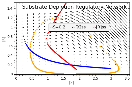
title = "Substrate Depletion Regulatory Network" ## Graph Title
xmin = 0 ## X minimum
xmax = 3.5 ## X maximum
ymin = 0 ## Y minimum
ymax = 1.5 ## Y maximum
## Add a title to the plot
g += text(title,(xmax/1.9,ymax*0.95),color='black',fontsize=15)
## Add the desired lines to the plot
g += plot_vector_field((r1.rhs(),r2.rhs()), (X,0,3.5), (R,0,1.3))
g += list_plot(sols_0,color='orange',legend_label='S=0.2')
g += list_plot(sols_1,color='blue',legend_label='[X]ss')
g += list_plot(sols_2,color='red',legend_label='[R]ss')
## For more information on plots in general, evaluate 'plot?'
## For a list of legend options, evaluate 'a.set_legend_options?'
## For a list of Sage predefined colors, evaluate 'sorted(colors)'
g.set_axes_range(xmin,xmax,ymin,ymax)
g.axes_labels(['[X]','[R]'])
g.axes_label_color('grey')
g.set_legend_options(ncol=3,borderaxespad=5,back_color='whitesmoke',fancybox=true)
show(g)
|
|
|