Sage Primer

Doug White

Merrimack College

Department of Physics

Intro:

Sage is a free open-source mathematics software system licensed under the GPL. It combines the power of many existing open-source packages into a common Python-based interface. Sage can be used to perform symbolic, algebraic, and numerical computations. Sage is used to study general and advanced, pure and applied mathematics,and is well suited for educational purposes.

The interface is a notebook in a web-browser or the command-line. Using the notebook, Sage connects either locally to your own Sage installation or to a Sage server on the network (as we are doing today). Inside the Sage notebook you can create embedded graphics, typeset mathematical expressions, add and delete input, and share your work across the network (.sws files). There are several very good tutorials on the Sage website including Sage for Newbies a book by T. Kosan, these tutorials are very helpful in learning to use the many features available in Sage. I found that a quick way to start learning Sage is to download and print the Quick Reference Cards which provide a brief overview of some of the more common functions with syntax.

The goal of this Primer is to give you some familiarity with the notebook interface and to provide several quick examples of using Sage as a calculator in the next half hour or so. The various tutorials and the Sage reference manual give a much more in depth look at Sage, in particular the fact that the interface is based on the Python programming language allows much more functionality than we will see today.

Sage is used for research in a wide range of fields including, algebra, calculus, number theory, cryptography, numerical computation, commutative algebra, group theory, combinatorics, graph theory, and linear algebra to name a few (see some online books using Sage and a list of publications using Sage).

Basics:

With sage it is simple to perform calculations, for example in the 'cell' below two numbers are added, $2 + 6$. (Note the red line next to the cell, this indicates the instructions within it have not been executed, it will disappear once they are.)

In order to evaluate this expression simply click on the cell and then click on 'evaluate' just below the expression or simply press <shift> + <enter> on the keyboard. Try it. The operations -, /, *, ^, refer to subtraction, division, multiplication, and exponentiation respectively. There are also many basic functions and constants available in Sage as illustrated in the cell below;

-4^2

-16

-16

Note that in the cell above we have separated various calculations with a semi-colon so each does not need its own cell.

Sage has built in documentation that gives the details on syntax, options available for each command, and examples. In order to show the documentation simply type the command name in a cell followed by a ? and push <tab>, so for example if we wanted to know more about the tanh function;

tanh?

File: /usr/local/sage2/local/lib/python2.6/site-packages/sage/functions/hyperbolic.py

Type: <class ‘sage.functions.hyperbolic.Function_tanh’>

Definition: tanh(*args, coerce=True, hold=False, dont_call_method_on_arg=False)

Docstring:

The hyperbolic tangent function.

EXAMPLES:

sage: tanh(pi)
tanh(pi)
sage: tanh(3.1415)
0.996271386633702
sage: float(tanh(pi))
0.996272076220749...
sage: tan(3.1415/4)
0.999953674278156
sage: tanh(pi/4)
tanh(1/4*pi)
sage: RR(tanh(1/2))
0.462117157260010

sage: CC(tanh(pi + I*e))
0.997524731976164 - 0.00279068768100315*I
sage: ComplexField(100)(tanh(pi + I*e))
0.99752473197616361034204366446 - 0.0027906876810031453884245163923*I
sage: CDF(tanh(pi + I*e))
0.997524731976 - 0.002790687681*I

To prevent automatic evaluation, use the hold parameter:

sage: tanh(arcsinh(x),hold=True)
tanh(arcsinh(x))

To then evaluate again, we currently must use Maxima via sage.symbolic.expression.Expression.simplify():

sage: tanh(arcsinh(x),hold=True).simplify()
x/sqrt(x^2 + 1)

TESTS:

sage: latex(tanh(x))
\tanh\left(x\right)

File: /usr/local/sage2/local/lib/python2.6/site-packages/sage/functions/hyperbolic.py

Type: <class ‘sage.functions.hyperbolic.Function_tanh’>

Definition: tanh(*args, coerce=True, hold=False, dont_call_method_on_arg=False)

Docstring:

The hyperbolic tangent function.

EXAMPLES:

sage: tanh(pi)
tanh(pi)
sage: tanh(3.1415)
0.996271386633702
sage: float(tanh(pi))
0.996272076220749...
sage: tan(3.1415/4)
0.999953674278156
sage: tanh(pi/4)
tanh(1/4*pi)
sage: RR(tanh(1/2))
0.462117157260010

sage: CC(tanh(pi + I*e))
0.997524731976164 - 0.00279068768100315*I
sage: ComplexField(100)(tanh(pi + I*e))
0.99752473197616361034204366446 - 0.0027906876810031453884245163923*I
sage: CDF(tanh(pi + I*e))
0.997524731976 - 0.002790687681*I

To prevent automatic evaluation, use the hold parameter:

sage: tanh(arcsinh(x),hold=True)
tanh(arcsinh(x))

To then evaluate again, we currently must use Maxima via sage.symbolic.expression.Expression.simplify():

sage: tanh(arcsinh(x),hold=True).simplify()
x/sqrt(x^2 + 1)

TESTS:

sage: latex(tanh(x))
\tanh\left(x\right)

Sage will also try to complete a command name for you if you type in a partial name and then push the <tab> key, for example;

spherical_

Traceback (click to the left of this block for traceback)
...
NameError: name 'spheri' is not defined

Traceback (most recent call last):
  File "<stdin>", line 1, in <module>
  File "_sage_input_7.py", line 10, in <module>
    exec compile(u'open("___code___.py","w").write("# -*- coding: utf-8 -*-\\n" + _support_.preparse_worksheet_cell(base64.b64decode("c3BoZXJp"),globals())+"\\n"); execfile(os.path.abspath("___code___.py"))
  File "", line 1, in <module>
    
  File "/tmp/tmpCcaJZQ/___code___.py", line 2, in <module>
    exec compile(u'spheri
  File "", line 1, in <module>
    
NameError: name 'spheri' is not defined

will return a list of possibilities including, the spherical bessel function, the sperhical harmonic function, and the spherical hankel function.

These few tips along with the quick reference sheet will go a long way in getting you started performing calculations in Sage. So let's look at a few examples, as you investigate these examples play around by changing the values of constants and function definitions.

Plotting and some calculus examples

Note that in the cell below anything following the #symbol is a comment and does not effect the calculation.

plot(sin(x)/x,x,-5*pi,5*pi) #plot of a function

Also of note in the example above is the use of the variable x. By default Sage recognizes x as a variable, if you wish to use another symbol as a variable it must be defined as such as in the example below.

y=var('y') plot(sin(y)/y,y,-5*pi,5*pi)

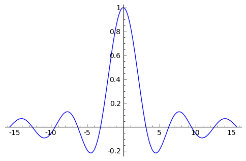
In the following cell the function numerical_integral is used to calculate $\int_{0}^{10} \frac{\sin x}{x} dx$.

numerical_integral(sin(x)/x,0,10) #numerical integral of the function from 0 to 10

(1.6583475942188737, 2.840710867141403e-14)

(1.6583475942188737, 2.840710867141403e-14)

It is simple to define functions in Sage as shown below. In the first line the function $f = \frac{\sin x}{x}$ (using the = sign) and then it is used in a calculation. Note that we can type two lower-case ohs, oo, as a shorthand for infinity.

f=sin(x)/x integral(f,-infinity,infinity)

pi

pi

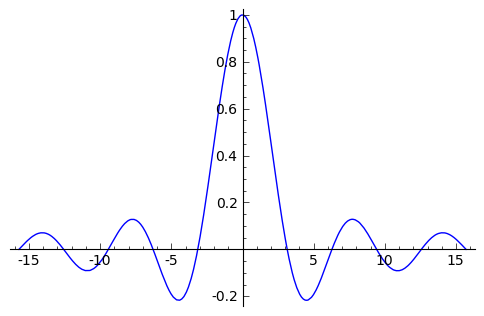
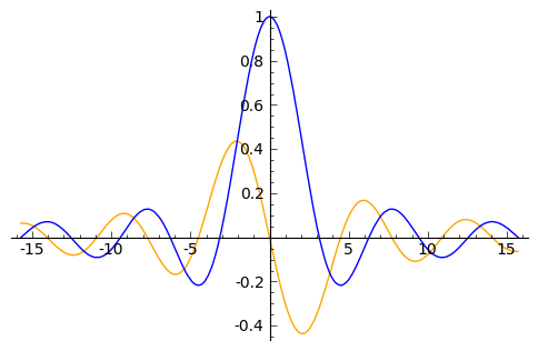
The first derivative of f with respect to x, $ \frac{df}{dx}$ is calculated and plotted below. Note we have used the option color to draw our plot in orange.

diff(f,x) #first derivative of the function wrt x.

cos(x)/x - sin(x)/x^2

cos(x)/x - sin(x)/x^2

plot(diff(f,x),x,-5*pi,5*pi,color="orange") + plot(f,x,-5*pi,5*pi) #note use of + to combine plots

Let's do some calculations using symbols. Below we define a and n as variables and then define the function $g=ax^n$.

a,n=var('a,n') #defines a and n as variables g=a*x^n #defines our function du jour

Now we calculate $\frac{dg}{dx}$ and $\frac{dg}{da}$.

diff(g,x); diff(g,a) #calculate dg/dx and dg/da

a*n*x^(n - 1)
x^n

a*n*x^(n - 1)
x^n

If you want the result to look a little better perhaps, try using the view function which will typeset your result using $\TeX$ another great open-source software package integrated with Sage. If you like you can type the following into a cell, pretty_print_default() ,and evaluate it, all of your output will then automatically typeset without having to use view every time.

view(diff(g,x)); view(diff(g,a))

\newcommand{\Bold}[1]{\mathbf{#1}}a n x^{{\left(n - 1\right)}}

\newcommand{\Bold}[1]{\mathbf{#1}}x^{n}

\newcommand{\Bold}[1]{\mathbf{#1}}a n x^{{\left(n - 1\right)}}

\newcommand{\Bold}[1]{\mathbf{#1}}x^{n}

Next let's calculate some limits. Below we calculate $\lim_{x \rightarrow 0} \frac{1}{x}$.

lim(1/x,x=0)

Infinity

Infinity

Sage is telling us that it cannot determine the result, however we can specify from which direction to take the limit and this will help.

lim(1/x,x=0,dir="right"); lim(1/x,x=0,dir="left")

+Infinity
-Infinity

+Infinity
-Infinity

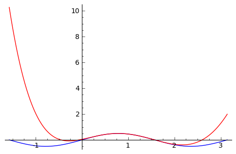
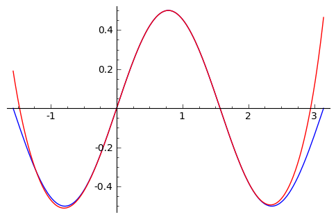
Now let's look at some Taylor series expansion of a function. In addition we will plot the Taylor polynomial with the function to get a graphical representation of how good the approximation is.

h(x)=sin(x)*cos(x) #define function h(x) i(x)=taylor(h(x),x,1,5) #taylor expansion of h(x) about x=1 to 5th order j(x)=taylor(h(x),x,1,8) #taylor expansion of h(x) about x=1 to 5th order

plot(h(x),x,-pi/2,pi) + plot(i(x),x,-pi/2,pi,color='red')

plot(h(x),x,-pi/2,pi)+plot(j(x),x,-pi/2,pi,color='red')

Very nice.

Some differential equations

The desolve function can be used to solve differential equations using Laplace transforms, in the example that follows a 1st order linear differential equation is solved. The first line defines t to be a variable, the second line defines x to be a function of the variable t, next the differential equation $\frac{dx}{dt} + 3x +1 = 0$ is defined. The desolve function is then used to solve for the dependent variable x as a function of the independent variable t.

t=var('t') x=function('x',t) de=diff(x,t)+3*x+1 soln=desolve(de,x) view(soln)

\newcommand{\Bold}[1]{\mathbf{#1}}\frac{1}{3} \, {\left(3 \, c - e^{\left(3 \, t\right)}\right)} e^{\left(-3 \, t\right)}

In the solution above the constant c can be determined if the initial conditions are known, for example below we solve the same differential equation and set the initial conditions to x=2 at t=0.

soln2=desolve(de,x,ics=[0,2]) view(soln2)

\newcommand{\Bold}[1]{\mathbf{#1}}-\frac{1}{3} \, {\left(e^{\left(3 \, t\right)} - 7\right)} e^{\left(-3 \, t\right)}

We can use the expand and simplify functions to manipulate algebraic expressions as illustrated below.

view(expand(soln2))

\newcommand{\Bold}[1]{\mathbf{#1}}\frac{7}{3} \, e^{\left(-3 \, t\right)} - \frac{1}{3}

plot(soln2,t,-.5,2)

We can use the find_root function to find when the function is equal to 0.

find_root(soln2,.5,1)

0.64863671635177067

0.64863671635177067

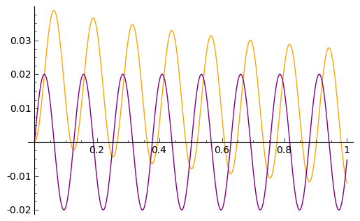
Here we solve the differential equation for a circuit with an inductor and resistor in series driven by an alternating voltage source.

A,B,w,t=var('A,B,w,t') # define the variables we will be using I=function('I',t) #identify I as a function of t, I is the current de=diff(I,t)+I-sin(50*t) # the differential equation ret=desolve(de,I,ics=[0,0],ivar=t) #solve for I using desolve function view(expand(ret)) #print the solution

\newcommand{\Bold}[1]{\mathbf{#1}}\frac{50}{2501} \, e^{\left(-t\right)} + \frac{1}{2501} \, \sin\left(50 \, t\right) - \frac{50}{2501} \, \cos\left(50 \, t\right)

Let's plot the current, to show phase shift we also plot a function with phase and frequency of voltage source (in purple). Also note the initial transient dying off.

plot(ret,t,0,1,color='orange')+plot(.02*sin(50*t),t,0,1,color='purple') #plot I vs. t

A little linear algebra

In the example below we will define a matrix and a vector and perform some calculations.

m=matrix([[1,2,3],[3,4,5],[-4,6,-2]]) m #define a matrix, then display it

[ 1  2  3]
[ 3  4  5]
[-4  6 -2]

[ 1  2  3]
[ 3  4  5]
[-4  6 -2]

transpose(m) #find the transpose of the matrix m

[ 1  3 -4]
[ 2  4  6]
[ 3  5 -2]

[ 1  3 -4]
[ 2  4  6]
[ 3  5 -2]

inv=m^(-1) ;inv #find the inverse of m

[-19/18  11/18  -1/18]
[ -7/18   5/18    1/9]
[ 17/18  -7/18  -1/18]

[-19/18  11/18  -1/18]
[ -7/18   5/18    1/9]
[ 17/18  -7/18  -1/18]

m*inv #Matrix multiplication, test whether or not inverse found

[1 0 0]
[0 1 0]
[0 0 1]

[1 0 0]
[0 1 0]
[0 0 1]

There are functions to find eigenvalues and eigenvectors of the matrix m...

m.eigenvalues() #returns the eigenvalues of matrix m

[-3, -1.582575694955840?, 7.582575694955840?]

[-3, -1.582575694955840?, 7.582575694955840?]

view(m.eigenvectors_right() ) #returns the eigenvalues, eigenvectors, and multiplicity

\newcommand{\Bold}[1]{\mathbf{#1}}\left[\left(-3, \left[\left(1,1,-2\right)\right], 1\right), \left(\hbox{-1.582575694955840?}, \left[\left(1,\hbox{0.579880962221226?},\hbox{-1.247445873132764?}\right)\right], 1\right), \left(\hbox{7.582575694955840?}, \left[\left(1,\hbox{2.020119037778775?},\hbox{0.8474458731327635?}\right)\right], 1\right)\right]

Solving a matrix equation can be done with the solve_right function.

w=vector([2,3,-2]) #define a vector w ans=m.solve_right(w) #solves the matrix equation, m*ans=w view(ans) #prints the solution

\newcommand{\Bold}[1]{\mathbf{#1}}\left(-\frac{1}{6},-\frac{1}{6},\frac{5}{6}\right)

Now let's verify the answer by testing whether or not the product of m and ans is equal to vector w. To do this we will use the == symbol (double equal sign), in Sage this symbol is used to compare one expression to another and will return either true or false. (The equal sign = is used for assignment so f=x^2 defines the function f as $x^2$, whereas f==x^2 means "are f and $x^2$ the same thing?)

m*ans==w #check our answer, should get vector w, the

True

True

3-d Plots

var('x,y') show(plot3d(sin(x)*cos(y), (x,-2*pi,2*pi), (y,-pi,pi), rgbcolor='purple',opacity=.9,mesh=true))

Try rotating the plot with the curser.

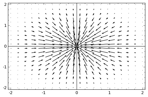
var('x,y') show(plot3d(x^2+cos(x)*y^2, (x,-5,5), (y,-5,5), color='orange',opacity=.86,mesh=true))

2-d vector field plots and gradient function

sage: u,v = var('u v') sage: f = exp(-(u^2+v^2)) sage: plot_vector_field(f.gradient(), (u,-2,2), (v,-2,2))

Introduction to SAGE

4223 days ago by comphy