
- 전체
- C/C++ 일반
- C/C++ 수학
- C/C++ 그래픽
- C/C++ 자료구조
- C/C++ 인공지능
- C/C++ 인터넷
- wxWidget
- GTK+
- UNIX or LINUX programming
- 리눅스 마스터 - 국가공인자격
- VC++/ MFC
- C#/CLI/.NET
- QT/기타UI
- Boost lib
- 오픈소스 C 분석자료
- MSA (마이크로서비스), Docker, kubernetes
- WSL(windows subsystem linux)
C/C++ 인공지능 [C/C++ 인공지능] A Simple and Complete Explanation of Neural Networks : 신경망에 대한 간단하고 완전한 설명
2023.10.22 13:57
[C/C++ 인공지능] A Simple and Complete Explanation of Neural Networks : 신경망에 대한 간단하고 완전한 설명
A Simple and Complete Explanation of Neural Networks

 98.6K
98.6K 1.2K
1.2K 86
86Introduction
Nowadays, scientists are trying to find power of human brain. They try to imitate it for finding big data solution.

I feel that there is no comprehensive, easy, clear and practical article on NN. I always wanted to know how the human brain works biologically. I had many questions that remained unanswered. Neural Network details was always ambiguous for me. The most important questions that I want to answer are:
- How Human Brain Works Exactly?
- How Perceptron as an Artificial Neuron Works - Forward Neural Network?
- What Is Weight in Neural Network?
- What Is Equivalent for Weight in Biological Neuron?
- What Is Activation Function Role in Neural Network?
- What Is Equivalent for Activation Function in Biological Neuron?
- How Backward Propagation Works?
- What Is the Exact Mathematical Logic for Backward Propagation Neural Network?
- How to Implement Backward Propagation Neural Network?
1. How Human Brain Works Exactly?
For understanding that how neural network works, it is better to study about human brain operation. There are approximately 1011 neurons inside brain which are highly connected to each other. When you see an animal for example cat, its features such as size, color and shape are entered to your brain from your eyes gate. Then, these input information will be calculated by small cells so called neurons that are responsible for processing input data in your brain.
Firstly, neurons search about your other images from cats which you have seen before. They compare between previous cat pictures in your memory and new cat. This comparison which is fundamental of supervised learning process has made your brain as a comparison tool. This is why human beings tend to compare everything. Finally, response is that you saw a cat because you had seen a cat in the past.
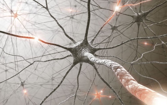
You can process 20 MB per second just with the aid of your optical sense and it is awesome because it is regardless of your abilities to learn something or to detect the voice of someone or your auditory capability. Therefore, your brain is an unbelievably huge CPU.
Assume that having much smaller scale of this huge system how much can solve nowadays problems in different areas and domains. For instance, very small portion of brain's features can solve issues in speech and face or image recognition, sentiment analysis and opinion or emotion reading, driving a car automatically or even disease diagnosis.
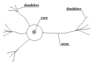
There is a neuron cell in the below picture, it includes dendrites, axon and core. Please look at it from left to right. Dendrites are responsible to receive information and its core is where data is processed and the result will be transmitted from axon to the tail of the neuron. The total structure of one of this neuron in artificial intelligence is called perceptron.
Another neuron cell on the right side will receive the response of the left side neuron with the aid of some chemical substances which cause fire. Its ignition causes to send and transfer data to other cells. So output from left side neuron is such as input for right side neuron. This process will happen for the rest of other cells. Therefore 1010 neurons in brain collaborate to reach their own goal.
Assume how many processes per day are there to analyze in order to handling your life. Brain performs all of them without much exhausting. At the end of the day, you just need 7 hours to cool these little cells. Neuroscientists found out that more learning can make your dendrites mush stronger, because igniting the connection between your neuron cells is a practice which is almost like exercising for your muscles. Therefore, using brain is less likely to get Alzheimers disease.
2. How Perceptron as an Artificial Neuron Works - Forward Neural Network?
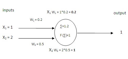
In the below picture, you can see one simple perceptron and its operation in order to compute its output. Firstly, there are two inputs as X1 X2, and then there are weights for each connection to node. In neural network, all of processing unit is the node and in spite of computer systems which have complex processing unit, in NN there is simple unit for processing. we multiply two numbers (X and weight).
Then we sum up all of X*weight and apply activation function on the result value and final output is perceptron answer.
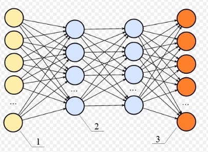
The whole story in the above paragraph is called as forward propagation in neural network. But indeed, we use more nodes and multiple layers for NN learning. I mentioned that in our brain, there are billions layers and that huge system made us as a human being today. So, for having better learning, we use more layers. It can almost guarantee result improvement in learning or training at NN. There are two hidden layers as light blue in the below picture. The computation for each node will happen like a simple perceptron.

3. What Is Weight in Neural Network?
Weight refers to the strength of connection between nodes. Unsigned value (without +, -) of weight depends on how nodes have power to connect to each other.
It can be positive or negative. Positive means it is more likely to transmit data and having strong connection among neurons while negative is vice versa. At the initialize point, we select weight randomly but for having reasonable result it is better to normalize input data as follow, X is input data:
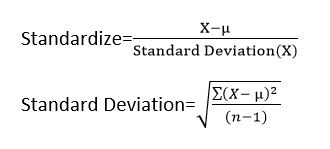
Because our activation function in this article is sigmoid. There is a shortcut solution to select weight as randomly is to determine our weight values in a specific range such as below formula which depends on uniform distribution which I keep its logic unspoken here and will extend it in the next article.
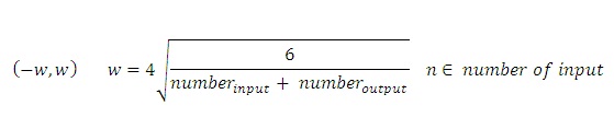
Reference for above formula is: Deep Learning Tutorials; Glorot and Bengio (2010)
I mentioned that neural network is highly interconnected and weight is the most valuable element which makes this connectivity. We select weight values randomly at the first phase. Firstly, forward propagation is done from left to right.
Then, make a comparison that how much output value is far from our real value. Real value is label which is “Y” in the training data set. Then backward propagation computation will be done, which performs computation in the inverse path.
Forward propagation is from left to right but back propagation is from right to left to optimize and gain new weight to enhance the next output. If the next output value has less difference from “Y” rather than previous output value, so, it shows us that we are in right direction.
So, weight is a tool to connect nodes to each other and a factor to train NN for having the less error. BP and FP and weights calibration will be measured repeatedly in order to obtain new values for weight and accurate output which decreases error.
For having the better understanding about weight role in NN, I invite you to read my article about “Machine Learning and Gradient Descent”. Weight in NN is almost something near to slope “a” in Yprediction line, Y = aX + b. Accurate value for “a” could help us to find better prediction line in order to classify our data. here in NN weight is also a factor such as “a“ and we struggle to find its value accurately to have more precision classification.
4. What Is Equivalent for Weight in Biological Neuron?
Everything in neural network structures is inspired from human brain. Therefore, unsigned values for weight means: dendrite connection between neurons + count of synapses between dendrites + pre and post synaptic terminals + gap shape among neurons + fusion intensity; last but not least is myelination.
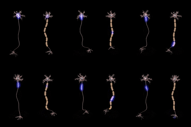
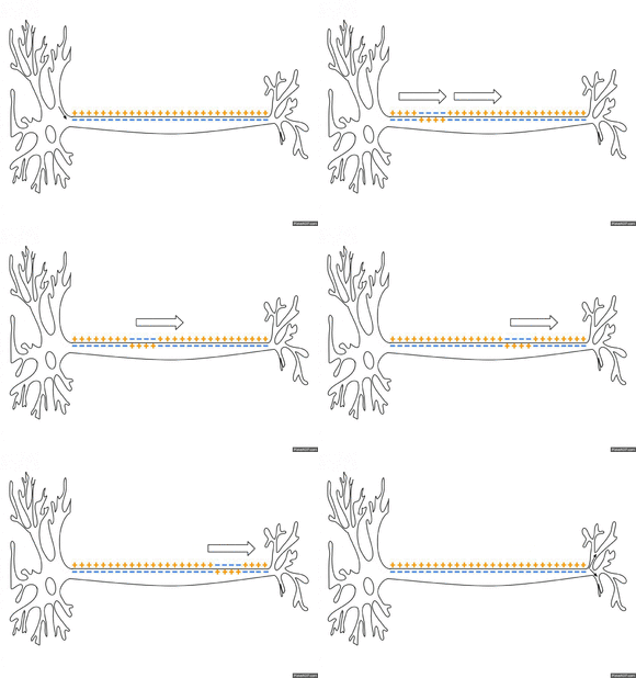
Myelination is white and fatty substance around axon of neuron cells and it is such as sheath or protector for them. On the below picture, propagation on the right neuron with myelination is much faster than left neuron without sheath. This phenomenon occurs because of saltatory conduction.
The number of propagation and its speed can make more and stronger synapses. These factors play important role to have better learning in our brain. Activity of Functional Magnetic Resonance Imaging - FMRI - in someone who has better functionality in their own brain shows that there are more synapses with more red points.
So, weight in neural network is as same as combination of above factors as biologically.
https://en.wikipedia.org/wiki/Myelin
5. What is Activation Function Role in Neural Network?
Activation function is (although a bit) equivalent to polarization and stabilizing. I want to bring an example as an introduction for polarization and making stabilizing in mathematic. For having easy computation, we need some polarizing on values especially decimal ones. For example, we have 1.298456 and we just need one number as decimal in order to round and polarizing and having easy and fast computation. We convert 1.298456 to 1.3 because the next number after 2 in decimal is 9 and it is more than 5 so we convert 2 into 3. In these cases, rounding can help to have more elegant values and results.
In neural network, we want to better distinguish and predict. So, non linear functions have more rounding and bending. Please look at the below picture. In comparison between linear and non linear functions, it is obvious that non linear is more accurate to predict and has better boundary decision line for categorizing between two different classes.
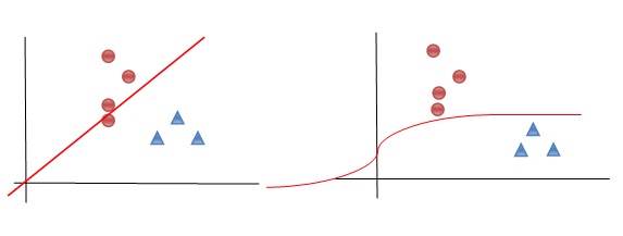
I used “Some Squared Error SSE” in the gradient descent. Activation function for neural network should be non linear function such as exponential or tangent and also it must be differentiable, because in the backward propagation, we need to find global minimum point. Indeed, backward propagation performs gradient descent. Please read the article about gradient descent with this link.
Sum of Squared Errors (SSE) = ½ Sum (Yactual– Ypredicted)2
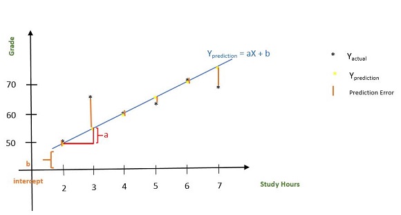
SSE measures error value between Yactual and Ypredicted. Therefore, for having best prediction line instead of blue line in the above picture, we differentiate SSE and compute new slope for this line.
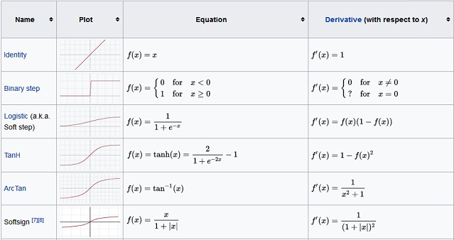
You can select one of below functions as your activation function. For reference, please look at this link.
6. What Is EquivaLent for Activation Function in Biological Neuron?
Activation function in neural network is called as transfer function. Transfer function in neural network makes output for nodes according to their own inputs. Activation function is called as action potential in biological which is related to how signals travel in axon.
The chemical substances make electrical ignition and cause to stimulate neurons and then its axon in order to transmit signal in just one direction of neuron. It helps to produce result for current neuron. For reference, please look at this link.
7. How Backward Propagation Works?
In order to sum up all of above concepts, I want to divide backward propagation in various steps as follows:
- There is training data set at the initial step which has one or more than one columns for X as input and one label as Y which should be read and considered. So, numbers of input and output layers are defined.
- We need to select number of hidden layers; count of hidden layers shows depth of learning. More hidden layers can imitate human brain better and enhance its accuracy. But the most important issue is that more hidden layers need more calculation especially in backward propagation and it consumes more memory.
- After hidden layers definition, we need weigh values which are selected randomly with Gaussian and there is formula that I have explained at third section of this article 3. What is weight in Neural Network?
*Forward Propagation to reach output value:
Each layer has node and I assume two values for them, first is without applying sigmoid function so called “Input_sigma” or “hidden_ sigma” and the next is with sigmoid function as “hidden_node”, “output_node”. Then we start computation from left to right for forward propagation.
Input_sigma = input_node * weight_1hidden_node = Sigmoid (input_sigma)hidden_sigma = hidden_node * weight_2Sigmoid (hidden_sigma) = output_nodemargin_error = expected – output_node*Backward Propagation to reach better weight:
In backward propagation because we need optimum value, we differentiate from sigmoid function and go inversely from right to left, in order to finding new values for weights.
output_node′ = Sigmoid′ (hidden_sigma) * marginweight_2 ′ = (output_node′ / hidden_node) + weight_2hidden_node ′ = (output_node′ / weight_2) * Sigmoid′ (input_sigma)weight_1 ′ = (hidden_node′ / input_node) + weight_1- Again, we repeat steps 1 to 5 with new weights and comparison value from current margin errors and previous margin errors if current error is less than previous one, so it shows us that we are in right direction.
- We iterate step 1 to 10 until margin error is near our “
Y”.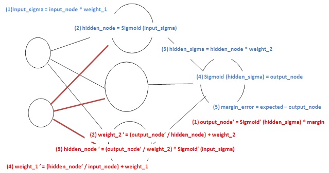
8. What Is the Exact Mathematical Logic for Backward Propagation Neural Network?
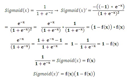
Backward propagation performs as same as gradient descent and we need to have differentiation of activation function. I described its computation as follows:
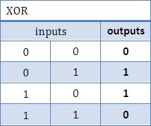
XOR is one simplest sample to test our first neural network. There is XOR table with two inputs and one output:
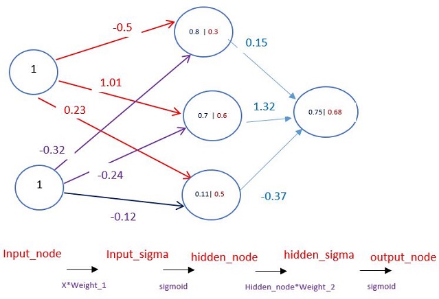
I want to implement fourth row in XOR which is (1, 1) = 0.
Y is 0 and output is 0.68. So margin error is -0.68. The next output is 0.57 which is less than 0.68.

9. How to Implement Backward Propagation Neural Network?
Execution File
According to all of the above explanation, I want to implement it on Matlab. Firstly, I created "execution.m" file for calling prediction function.
%% Machine Learning -  Neural Networks  - Simple Example

%% Initialization
clear ; close all; clc

input_node = [1 1]; %1*2

% Generate Weight By Gausian Distribution
Weight_1 = [ -0.5 1.01  0.23 ; -0.32 -0.24 -0.12 ]; %2*3
Weight_2 = [ 0.15 1.32 -0.37 ]; %1*3
pred = mypredict(Weight_1, Weight_2, input_node);
fprintf('\Final Output Backward Propagation: %f\n', perd);
Prediction File
Then I wrote "myprerdict.m" of which the most code will happen there:
function p = mypredict(Weight_1, Weight_2, input_node)

%Forward Propagation
input_sigma = input_node*Weight_1;
hidden_node = sigmoid(input_sigma); % 1*3
hidden_sigma = hidden_node*Weight_2';
output_node = sigmoid(hidden_sigma);

for jj=1:1000
    %sigmoid' = f(x)(1-f(x))
    %output_node_prime = s'(inner_sigma)*margin
    if jj>1
        Weight_2 = Weight_2_prime;
        Weight_1 = Weight_1_prime;
    end
        margin = 0 - output_node;
        sigmoid_prime_hidden_sigma = sigmoid(hidden_sigma);
        output_node_prime =
            (sigmoid_prime_hidden_sigma *(1-sigmoid_prime_hidden_sigma))*margin;

        delta_weight = (output_node_prime)./hidden_node; % 1*3
        Weight_2_prime = Weight_2 + delta_weight;

        sigmoid__prime_input_sigma = sigmoid_derivative(input_sigma);
        mydivide = output_node_prime./Weight_2;
        hidden_node_prime = zeros(1,3);
        hidden_node_prime(1,1) = mydivide(1,1) * sigmoid__prime_input_sigma(1,1);
        hidden_node_prime(1,2) = mydivide(1,2) * sigmoid__prime_input_sigma(1,2);
        hidden_node_prime(1,3) = mydivide(1,3) * sigmoid__prime_input_sigma(1,3);

        delta_weight_2 = hidden_node_prime'*input_node;

        Weight_1_prime = Weight_1 + delta_weight_2';

        input_sigma = input_node*Weight_1_prime;
        hidden_node = sigmoid(input_sigma); % 1*3
        hidden_sigma = hidden_node*Weight_2_prime';
        output_node = sigmoid(hidden_sigma);
end

p = output_node;

end
Sigmoid Function
function y = sigmoid(x)

y = 1.0 ./ (1.0 + exp(-x));

end
sigmoid_derivative
function y = sigmoid_derivative(x)

 %sigmoid' = f(x)*(1-f(x))

 sigmoid_helper_2 = zeros(1,3);
    for i=1:3
        a= x(1,i);
        sigmoid_helper_2(1,i)= sigmoid(a)*(1-sigmoid(a));
    end
 y = sigmoid_helper_2;

end
Points of Interest
I found Neural Network very exciting, I think we can call it as the mother of artificial intelligence.
The most advantages and disadvantages of NN are that:
- Normalizing data set and having best feature selections can lead us to have better accurate output in huge training data set.
- Performance and accuracy depends on weight but if you select it in correct range. then you can enhance performance and accuracy.
- Backward propagation consumes more memory than other ways.
Finally, I strongly recommend you to register machine learning in coursera.org: https://www.coursera.org/learn/machine-learning & use my github as guidance for assignments:
https://github.com/Hassankashi?tab=repositories
Feedback
Feel free to leave any feedback on this article; it is a pleasure to see your opinions and vote about this code. If you have any questions, please do not hesitate to ask me here.
History
- 3rd April, 2019: Initial version
License
This article, along with any associated source code and files, is licensed under The Code Project Open License (CPOL)

 Iran (Islamic Republic of)
I`d like to challenge with complex problem, then make it easy for using everyone. This is the best joy.
ICT Master in Norway 2013
Doctorandin at Technische Universität Berlin in Data Scientist ( currently )
-------------------------------------------------------------
Diamond is nothing except the pieces of the coal which have continued their activities finally they have become Diamond.
http://www.repocomp.com/


신경망에 대한 간단하고 완전한 설명
소개
요즘 과학자들은 인간 두뇌의 힘을 찾으려고 노력하고 있습니다. 빅데이터 솔루션을 찾기 위해 이를 모방하려고 합니다.
NN에 관한 포괄적이고, 쉽고, 명확하고, 실용적인 기사는 없다고 생각합니다. 나는 항상 인간의 뇌가 생물학적으로 어떻게 작동하는지 알고 싶었습니다. 나는 답을 얻지 못한 채 많은 질문을 갖고 있었습니다. 신경망 세부 사항은 나에게 항상 모호했습니다. 제가 대답하고 싶은 가장 중요한 질문은 다음과 같습니다.
- 인간의 두뇌는 정확히 어떻게 작동합니까?
- 인공 뉴런으로서의 퍼셉트론은 어떻게 작동합니까 - 순방향 신경망?
- 신경망에서 가중치란 무엇입니까?
- 생물학적 뉴런의 무게에 해당하는 것은 무엇입니까?
- 신경망에서 활성화 기능 역할이란 무엇입니까?
- 생물학적 뉴런의 활성화 기능과 동등한 것은 무엇입니까?
- 역방향 전파는 어떻게 작동합니까?
- 역전파 신경망의 정확한 수학적 논리는 무엇입니까?
- 역전파 신경망을 구현하는 방법은 무엇입니까?
1. 인간의 두뇌는 정확히 어떻게 작동하는가?
신경망이 어떻게 작동하는지 이해하려면 인간의 뇌 작동에 대해 연구하는 것이 좋습니다. 뇌 내부에는 약 10 11 개의 뉴런이 서로 밀접하게 연결되어 있습니다 . 예를 들어 고양이와 같은 동물을 보면 크기, 색깔, 모양과 같은 특징이 눈의 문을 통해 뇌로 입력됩니다. 그런 다음 이러한 입력 정보는 뇌의 입력 데이터 처리를 담당하는 뉴런이라고 불리는 작은 세포에 의해 계산됩니다.
첫째, 뉴런은 이전에 본 고양이의 다른 이미지를 검색합니다. 기억 속에 있는 이전 고양이 사진과 새 고양이 사진을 비교합니다. 지도 학습 과정의 기본인 이러한 비교는 여러분의 두뇌를 비교 도구로 만들었습니다. 이것이 바로 인간이 모든 것을 비교하려는 경향이 있는 이유입니다. 마지막으로 과거에 고양이를 본 적이 있어서 고양이를 보았다는 반응이 나왔습니다.
광학 감각의 도움으로 초당 20MB를 처리할 수 있으며 이는 무언가를 배우는 능력이나 누군가의 목소리를 감지하는 능력 또는 청각 능력과 관계가 없기 때문에 정말 좋습니다. 그러므로 당신의 두뇌는 믿을 수 없을 정도로 거대한 CPU입니다.
이 거대한 시스템의 규모가 훨씬 작아지면 오늘날 다양한 영역과 영역의 문제를 얼마나 해결할 수 있다고 가정해 보십시오. 예를 들어, 뇌의 기능 중 아주 작은 부분이 음성, 얼굴 또는 이미지 인식, 정서 분석 및 의견 또는 감정 읽기, 자동 운전, 질병 진단 등의 문제를 해결할 수 있습니다.
아래 그림에는 뉴런 세포가 있는데, 여기에는 수상돌기, 축삭 및 핵이 포함되어 있습니다. 왼쪽에서 오른쪽으로 봐주세요. 수상돌기는 정보를 수신하는 역할을 하며 그 핵심은 데이터가 처리되고 결과가 축삭에서 뉴런의 꼬리로 전송되는 곳입니다. 인공지능에서 이 뉴런 중 하나의 전체 구조를 퍼셉트론이라고 합니다.
오른쪽에 있는 또 다른 뉴런 세포는 화재를 일으키는 일부 화학 물질의 도움으로 왼쪽 뉴런의 반응을 받게 됩니다. 점화로 인해 데이터를 다른 셀로 보내고 전송하게 됩니다. 따라서 왼쪽 뉴런의 출력은 오른쪽 뉴런의 입력과 같습니다. 이 프로세스는 나머지 다른 셀에서도 발생합니다. 따라서 뇌의 1010개 뉴런은 서로 협력하여 자신의 목표를 달성합니다.
당신의 삶을 처리하기 위해 하루에 얼마나 많은 프로세스를 분석해야 하는지 가정해 보세요. Brain은 별로 지치지 않고 이 모든 것을 수행합니다. 결국, 이 작은 세포를 식히는 데 7시간만 있으면 됩니다. 신경과학자들은 더 많은 학습을 통해 수상돌기가 더 강해질 수 있다는 사실을 발견했습니다. 왜냐하면 뉴런 세포 사이의 연결을 활성화하는 것은 근육 운동과 거의 유사한 연습이기 때문입니다. 그러므로 뇌를 사용하면 알츠하이머병에 걸릴 확률이 낮아집니다.
2. 인공 뉴런으로서의 퍼셉트론은 어떻게 작동합니까 - 순방향 신경망?
아래 그림에서는 출력을 계산하기 위한 하나의 간단한 퍼셉트론과 그 작동을 볼 수 있습니다. 먼저 X1 X2라는 두 개의 입력이 있고 노드에 대한 각 연결에 대한 가중치가 있습니다. 신경망에서는 모든 처리 단위가 노드이고, 컴퓨터 시스템은 복잡한 처리 단위를 가지고 있음에도 불구하고 NN에서는 처리를 위한 간단한 단위가 있다. 두 숫자(X와 가중치)를 곱합니다.
그런 다음 X*weight를 모두 합산하고 결과 값에 활성화 함수를 적용하면 최종 출력은 퍼셉트론 응답이 됩니다.
위 단락의 전체 이야기를 신경망에서는 순전파(forward propagation)라고 합니다. 그러나 실제로 우리는 NN 학습을 위해 더 많은 노드와 여러 레이어를 사용합니다. 우리 뇌에는 수십억 개의 층이 있고 그 거대한 시스템이 오늘날의 우리를 인간으로 만들었다고 말씀드렸습니다. 따라서 더 나은 학습을 위해 더 많은 레이어를 사용합니다. NN에서의 학습이나 훈련 결과 개선을 거의 보장할 수 있습니다. 아래 그림에는 하늘색으로 표시된 히든 레이어가 2개 있습니다. 각 노드에 대한 계산은 단순한 퍼셉트론처럼 발생합니다.
3. 신경망에서 가중치란 무엇입니까?
가중치는 노드 간의 연결 강도를 나타냅니다. 가중치의 부호 없는 값(+, - 제외)은 노드가 서로 연결되는 전력을 어떻게 보유하는지에 따라 달라집니다.
긍정적일 수도 있고 부정적일 수도 있습니다. 긍정적인 것은 데이터를 전송할 가능성이 더 높고 뉴런 사이에 강한 연결을 가질 가능성이 있다는 것을 의미하고 부정적인 것은 그 반대의 경우도 마찬가지입니다. 초기화 지점에서 가중치를 무작위로 선택하지만 합리적인 결과를 얻으려면 다음과 같이 입력 데이터를 정규화하는 것이 좋습니다. X는 입력 데이터입니다.
이 글의 활성화 함수는 시그모이드이기 때문입니다. 무작위로 가중치를 선택하는 간단한 솔루션은 균일 분포에 의존하는 아래 공식과 같은 특정 범위의 가중치 값을 결정하는 것입니다. 여기서는 해당 논리를 말하지 않고 다음 기사에서 확장할 것입니다.
위 공식에 대한 참고 자료는 Deep Learning Tutorials입니다. 글로롯과 벤지오(2010)
저는 신경망이 상호 연결되어 있고 무게가 이러한 연결을 만드는 가장 중요한 요소라고 언급했습니다. 첫 번째 단계에서는 가중치 값을 무작위로 선택합니다. 첫째, 순방향 전파는 왼쪽에서 오른쪽으로 수행됩니다.
그런 다음 출력 값이 실제 값과 얼마나 떨어져 있는지 비교하십시오. Y실제 값은 훈련 데이터 세트에서 " "인 레이블입니다 . 그런 다음 역전파 계산이 수행되어 역경로에서 계산이 수행됩니다.
순방향 전파는 왼쪽에서 오른쪽으로 이루어지지만 역전파는 최적화하고 다음 출력을 향상시키기 위해 새로운 가중치를 얻기 위해 오른쪽에서 왼쪽으로 이루어집니다. 다음 출력값이 Y이전 출력값보다 “ ”과의 차이가 적다면 올바른 방향으로 가고 있음을 알 수 있습니다.
따라서 가중치는 노드를 서로 연결하는 도구이자 오류가 덜하도록 NN을 훈련시키는 요소입니다. BP, FP 및 중량 교정은 중량에 대한 새로운 값과 오류를 줄이는 정확한 출력을 얻기 위해 반복적으로 측정됩니다.
NN의 가중치 역할에 대해 더 잘 이해하려면 "기계 학습 및 경사하강법"에 대한 내 기사를 읽어 보시기 바랍니다. NN의 가중치는 Y 예측 선의 기울기 "a"(Y = aX + b) 에 거의 가깝습니다 . "a"의 정확한 값은 데이터를 분류하기 위해 더 나은 예측선을 찾는 데 도움이 될 수 있습니다. 여기 NN 가중치는 "a"와 같은 요소이기도 하며 보다 정밀한 분류를 위해 해당 값을 정확하게 찾는 데 어려움을 겪습니다.
4. 생물학적 뉴런의 무게는 무엇입니까?
신경망 구조의 모든 것은 인간의 두뇌에서 영감을 받았습니다. 따라서 가중치에 대한 부호 없는 값은 다음을 의미합니다. 뉴런 사이의 수상돌기 연결 + 수상돌기 사이의 시냅스 수 + 시냅스 전후 말단 + 뉴런 간의 간격 모양 + 융합 강도; 마지막으로 중요한 것은 수초화입니다.
수초화란 신경세포의 축색돌기 주변에 있는 흰색의 지방성 물질로 신경세포의 외피나 보호막과 같은 역할을 합니다. 아래 그림에서 수초가 있는 오른쪽 뉴런의 전파는 덮개가 없는 왼쪽 뉴런보다 훨씬 빠릅니다. 이 현상은 도약 전도 때문에 발생합니다.
전파 횟수와 속도에 따라 시냅스가 더 많고 더 강력해질 수 있습니다. 이러한 요소들은 우리 뇌에서 더 나은 학습을 하는 데 중요한 역할을 합니다. 기능성 자기공명영상(Functional Magnetic Resonance Imaging, FMRI)의 활동은 자신의 뇌에 더 나은 기능을 가진 사람의 경우 더 많은 빨간색 점이 있는 시냅스가 더 많다는 것을 보여줍니다.
따라서 신경망의 가중치는 생물학적으로 위의 요소들의 조합과 동일합니다.
https://en.wikipedia.org/wiki/Myelin
5. 신경망에서 활성화 함수 역할이란 무엇입니까?
활성화 기능은 (약간이지만) 편광 및 안정화와 동일합니다. 저는 수학에서 양극화와 안정화를 위한 입문으로 예를 들고 싶습니다. 계산을 쉽게 하려면 값, 특히 소수 값에 대한 양극화가 필요합니다. 예를 들어, 1.298456이 있고 반올림 및 편파화하고 쉽고 빠른 계산을 위해서는 소수점으로 하나의 숫자만 필요합니다. 1.298456을 1.3으로 변환합니다. 왜냐하면 십진수 2 다음의 숫자는 9이고 5보다 크므로 2를 3으로 변환합니다. 이러한 경우 반올림은 더 우아한 값과 결과를 얻는 데 도움이 될 수 있습니다.
신경망에서는 더 나은 구별과 예측을 원합니다. 따라서 비선형 함수에는 반올림과 굽힘이 더 많습니다. 아래 그림을 봐주세요. 선형 함수와 비선형 함수를 비교할 때, 비선형 함수가 예측하기에 더 정확하고 서로 다른 두 클래스를 분류하는 데 있어 더 나은 경계 결정 라인을 갖는다는 것이 분명합니다.
경사하강법에서는 " Some Squared Error SSE "를 사용했습니다 . 신경망의 활성화 함수는 지수나 탄젠트와 같은 비선형 함수여야 하며, 역전파에서는 전역 최소점을 찾아야 하기 때문에 미분 가능해야 합니다. 실제로 역방향 전파는 경사하강법을 수행합니다. 이 링크를 통해 경사하강법에 대한 기사를 읽어보세요 .
SSE(제곱 오류 합계) = ½ 합계(Y 실제 – Y 예측 ) 2
YactualSSE는 과 사이의 오류 값을 측정합니다 Ypredicted. 따라서 위 그림의 파란색 선 대신 최상의 예측 선을 갖기 위해 SSE를 차별화하고 이 선에 대한 새로운 기울기를 계산합니다.
아래 기능 중 하나를 활성화 기능으로 선택할 수 있습니다. 참고로 이 링크를 살펴보시기 바랍니다 .
6. 생물학적 뉴런의 활성화 기능과 동등한 것은 무엇입니까?
신경망의 활성화 함수를 전달 함수라고 합니다. 신경망의 전달 함수는 노드 자체의 입력에 따라 출력을 생성합니다. 활성화 기능은 생물학적으로 활동 전위라고 불리며 축삭에서 신호가 어떻게 이동하는지와 관련이 있습니다.
화학 물질은 전기적 점화를 일으키고 뉴런과 그 축삭을 자극하여 뉴런의 한 방향으로만 신호를 전달합니다. 이는 현재 뉴런에 대한 결과를 생성하는 데 도움이 됩니다. 참고로 이 링크를 살펴보시기 바랍니다 .
7. 역전파는 어떻게 작동하는가?
위의 모든 개념을 요약하기 위해 역방향 전파를 다음과 같이 다양한 단계로 나누고 싶습니다.
- 초기 단계에는 입력으로 X에 대한 하나 이상의 열이 있고 읽고 고려해야 하는 Y에 대한 하나의 레이블이 있는 훈련 데이터 세트가 있습니다. 따라서 입력 및 출력 레이어의 수가 정의됩니다.
- 숨겨진 레이어 수를 선택해야 합니다. 숨겨진 레이어의 수는 학습의 깊이를 나타냅니다. 숨겨진 레이어가 많을수록 인간의 두뇌를 더 잘 모방하고 정확도를 높일 수 있습니다. 그러나 가장 중요한 문제는 특히 역방향 전파에서 더 많은 숨겨진 레이어가 더 많은 계산을 필요로 하고 더 많은 메모리를 소비한다는 것입니다.
- 히든 레이어 정의 후에는 가우시안을 사용하여 무작위로 선택된 가중치 값이 필요하며 이 기사의 세 번째 섹션에서 설명한 공식이 있습니다. 3. 신경망에서 가중치란 무엇입니까?
* 출력 값에 도달하기 위한 순방향 전파:
Input_sigma각 레이어에는 노드가 있고 이에 대해 두 가지 값을 가정합니다. 첫 번째는 " " 또는 " " 라고 하는 시그모이드 함수를 적용하지 않고 hidden_ sigma다음은 " hidden_node", " output_node"와 같은 시그모이드 함수를 사용하는 것입니다. 그런 다음 순방향 전파를 위해 왼쪽에서 오른쪽으로 계산을 시작합니다.
Input_sigma = input_node * weight_1hidden_node = Sigmoid (input_sigma)hidden_sigma = hidden_node * weight_2Sigmoid (hidden_sigma) = output_nodemargin_error = expected – output_node* 더 나은 가중치에 도달하기 위한 역전파:
역전파에서는 최적의 값이 필요하기 때문에 시그모이드 함수를 미분하고 오른쪽에서 왼쪽으로 역전파하여 새로운 가중치 값을 찾습니다.
output_node′ = Sigmoid′ (hidden_sigma) * marginweight_2 ′ = (output_node′ / hidden_node) + weight_2hidden_node ′ = (output_node′ / weight_2) * Sigmoid′ (input_sigma)weight_1 ′ = (hidden_node′ / input_node) + weight_1- 이번에도 현재 오류가 이전 마진 오류보다 작으면 현재 마진 오류와 이전 마진 오류로부터 새로운 가중치와 비교 값을 사용하여 1~5단계를 반복하므로 올바른 방향으로 가고 있음을 알 수 있습니다.
- 마진 오류가 " "에 가까워질 때까지 1~10단계를 반복합니다
Y.
8. 역전파 신경망의 정확한 수학적 논리는 무엇입니까?
역방향 전파는 경사하강법과 동일하게 수행되며 활성화 함수를 차별화해야 합니다. 나는 그 계산을 다음과 같이 설명했습니다.
XOR은 첫 번째 신경망을 테스트하는 가장 간단한 샘플 중 하나입니다. 두 개의 입력과 하나의 출력이 있는 XOR 테이블이 있습니다.
XOR에서 네 번째 행을 구현하고 싶습니다 (1, 1) = 0.
Y는 0이고 출력은 0.68입니다. 따라서 마진 오류는 -0.68입니다. 다음 출력은 0.57로 0.68보다 작습니다.
9. 역전파 신경망을 구현하는 방법은 무엇입니까?
실행 파일
위의 모든 설명에 따르면 Matlab에서 구현하고 싶습니다. 먼저 예측 함수를 호출하기 위한 " execution.m " 파일을 만들었습니다 .
%% 기계 학습 - 신경망 - 간단한 예

%% 초기화
분명한 ; 모두 닫습니다. 클씨

input_node = [ 1  1 ]; %1* 2

% 가우스 분포에 따른 가중치 생성
Weight_1 = [ - 0 . 5  1 . 01   0 . 23 ; - 0 . 32-0 . _ _ 24-0 . _ _ 12 ]; %2* 3
Weight_2 = [ 0 . 15  1 . 32-0 . _ _ 37 ]; %1* 3
pred = mypredict(Weight_1, Weight_2, input_node);
fprintf( ' \최종 출력 역방향 전파: %f\n' , perd);
예측 파일
그런 다음 " myprerdict.m "을 작성했는데 그 중 대부분의 코드가 여기에서 발생합니다.
함수 p = mypredict(Weight_1, Weight_2, input_node)

%순방향 전파
input_sigma = input_node*Weight_1;
Hidden_node = 시그모이드(input_sigma); % 1 * 3
Hidden_sigma = Hidden_node*Weight_2';
출력 노드 = 시그모이드(hidden_sigma);

jj=1:1000 의 경우
    %시그모이드 ' = f(x)(1-f(x))
    %output_node_prime = s' (inner_sigma)*
     jj > 1 인 경우 마진
        Weight_2 = Weight_2_prime;
        Weight_1 = Weight_1_prime;
    끝
        마진 = 0 - 출력_노드;
        sigmoid_prime_hidden_sigma = 시그모이드(hidden_sigma);
        출력_노드_프라임=
            (sigmoid_prime_hidden_sigma *( 1 -sigmoid_prime_hidden_sigma))*마진;

        delta_weight = (output_node_prime)./hidden_node; % 1 * 3
        Weight_2_prime = Weight_2 + delta_weight;

        sigmoid__prime_input_sigma = sigmoid_derivative(input_sigma);
        mydivide = output_node_prime./Weight_2;
        Hidden_node_prime = 0( 1 , 3 );
        Hidden_node_prime( 1 , 1 ) = mydivide( 1 , 1 ) * sigmoid__prime_input_sigma( 1 , 1 );
        Hidden_node_prime( 1 , 2 ) = mydivide( 1 , 2 ) * sigmoid__prime_input_sigma( 1 , 2 );
        Hidden_node_prime( 1 , 3 ) = mydivide( 1 , 3 ) * sigmoid__prime_input_sigma( 1 , 3 );

        delta_weight_2 = Hidden_node_prime ' *input_node;

        Weight_1_prime = Weight_1 + delta_weight_2' ;

        input_sigma = input_node*Weight_1_prime;
        Hidden_node = 시그모이드(input_sigma); % 1 * 3
        Hidden_sigma = 숨겨진_노드*Weight_2_prime ' ;
        출력 노드 = 시그모이드(hidden_sigma);
끝

p = 출력_노드;

끝
시그모이드 함수
함수 y = 시그모이드(x)

y = 1 . 0 ./( 1 . 0 + exp(-x));

끝
시그모이드_미분
함수 y = 시그모이드_미분(x)

 %시그모이드 ' = f(x)*(1-f(x))

 sigmoid_helper_2 = zeros(1,3);
    i=1:3의 경우
        a= x(1,i);
        sigmoid_helper_2(1,i)= 시그모이드(a)*(1-sigmoid(a));
    끝
 y = 시그모이드_헬퍼_2;

끝
가볼만한 곳
저는 Neural Network를 매우 흥미롭게 생각했습니다. 인공지능의 어머니라고 부를 수 있을 것 같습니다.
NN의 가장 큰 장점과 단점은 다음과 같습니다.
- 데이터 세트를 정규화하고 최상의 기능을 선택하면 대규모 훈련 데이터 세트에서 더 정확한 결과를 얻을 수 있습니다.
- 성능과 정확도는 무게에 따라 다르지만 올바른 범위에서 선택하는 경우. 그러면 성능과 정확성을 향상시킬 수 있습니다.
- 역방향 전파는 다른 방법보다 더 많은 메모리를 소비합니다.
마지막으로, Coursera.org( https://www.coursera.org/learn/machine-learning )에 기계 학습을 등록하고 과제 지침으로 제 github을 사용하는 것을 강력히 권장합니다.
https://github.com/Hassankashi?tab=repositories
피드백
이 기사에 대한 의견을 자유롭게 남겨주세요. 이 코드에 대한 여러분의 의견을 보고 투표 하게 되어 기쁩니다 . 궁금한 점이 있으시면 주저하지 마시고 여기로 문의해 주세요.
역사
- 2019년 4월 3 일 : 초기 버전
특허
이 기사는 관련 소스 코드 및 파일과 함께 The Code Project Open License(CPOL) 에 따라 라이센스가 부여됩니다.
복잡한 문제에 도전해보고, 누구나 쉽게 사용할 수 있도록 만들고 싶습니다. 이것이 최고의 기쁨입니다.
노르웨이 ICT 석사 2013
베를린 공과대학 데이터 과학자 박사 (현재)
---------------------------------- --------------
다이아몬드는 다름 아닌 석탄 조각들이 활동을 계속해 마침내 다이아몬드가 된 것입니다.
http://www.repocomp.com/
광고 클릭에서 발생하는 수익금은 모두 웹사이트 서버의 유지 및 관리, 그리고 기술 콘텐츠 향상을 위해 쓰여집니다.
댓글 0
| 번호 | 제목 | 글쓴이 | 날짜 | 조회 수 |
|---|---|---|---|---|
| 2 |
[C/C++][gnuplot][수학][MFC] Windows 환경의 C++ 언어에서 gnuplot을 사용한 그래프 출력 2
 | 졸리운_곰 | 2021.11.12 | 735 |
| 1 |
[C/C++][gnuplot][수학][MFC] Windows 환경의 C++ 언어에서 gnuplot을 사용한 그래프 출력
| 졸리운_곰 | 2021.11.12 | 1835 |