• Download NeuralNetwork class source files - 3 KB
• Download CounterNeuralNetwork source files - 6 KB
• Download DigitsNeuralNetwork source files - 117 KB

NeuralNetwork_src.zip CounterNeuralNetwork_src.zip DigitsNeuralNetwork_src.zip

Contents

• Background
• Introduction
• Neural Network Class
  • forward
  • backward
  • train
  • test
  • evaluate
• Use Cases
  • Simple Counter
    • Train network
    • Test network
    • Save network
  • Handwritten Digits Recognition
    • Network architecture
    • Activity diagram
    • Used libraries
    • Training and testing
    • Save network
    • Evaluation
• History

Background

This article is not to explain the scientific side of (ANN) Artificial Neural Networks. It provides a simple C++ class without any complications in the mathematical calculations of the backpropagation algorithm. If you have good experience about ANN, you can skip to the next section, else, you can revise this very good resources about ANN. I have provided two use cases to facilitate code usage as much as possible.

• Introduction to Neural Networks
• Neural Network Applications
• Backpropagation Mathematics
• Backpropagation Algorithm

Introduction

Today, (ANN) Artificial neural networks has become dominant in many areas of life, whether an industry or at home. ANN enables machines to learn and to simulate human brain to recognize patterns, and make predictions as well as solve problems in every business sector. Smartphones and computers that we use on a daily basis are using ANN in some of its applications. For example, Finger Print and Face unlock services in smartphones and computers use ANN. Handwritten Signature Verification uses ANN. I have written a simple implementation for an Artificial Neural Network C++ class that handles backpropagation algorithm. The code depends on Eigen open-source templates to handle Matrices’ mathematics. I made code simple and fast as possible.

NeuralNetwork Class

NeuralNetwork is a simple C++ class with the following structure:

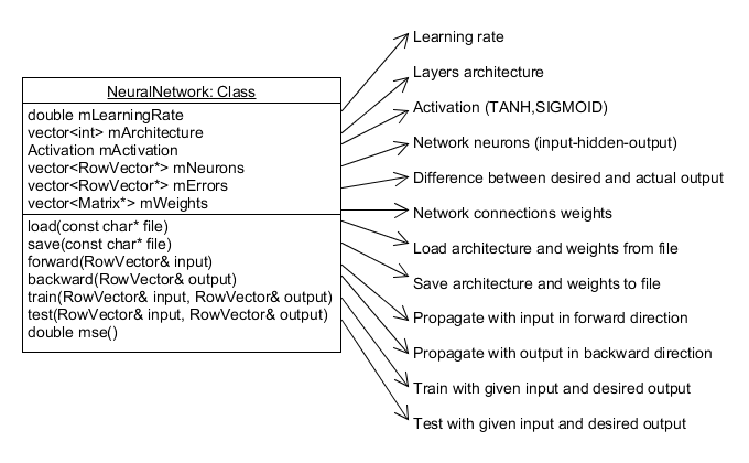
The code uses RowVectorXd and MatrixXd from Eigen template library. The main functions "train" and "test" take input and desired output in RowVector format. Both of them call "forward" function which uses vector multiplication.

forward

void NeuralNetwork::forward(RowVector& input) {
    // set first layer input
    mNeurons.front()->block(0, 0, 1, input.size()) = input;

    // propagate forward (vector multiplication)
    for (unsigned int i = 1; i < mArchitecture.size(); i++) {
        // copy values ingoring last neuron as it is a bias
        mNeurons[i]->block(0, 0, 1, mArchitecture[i]) = 
            (*mNeurons[i - 1] * *mWeights[i - 1]).block(0, 0, 1, mArchitecture[i]);
        for (int col = 0; col < mArchitecture[i]; col++)
            mNeurons[i]->coeffRef(col) = activation(mNeurons[i]->coeffRef(col));
    }
}

The function propagates with input through network layers to get output from the last layer. Each neuron in the hidden layer first computes a weighted sum of its inputs. Then it applies an activation function (segmoid) to this sum to derive its output. This function affects neurons values only. It doesn't affect connections weights or errors. This function does this sum with vector multiplication:

(*mNeurons[i - 1] * *mWeights[i - 1])

Then, resultant values are passed through activation function.

double NeuralNetwork::activation(double x) {
    if (mActivation == TANH)
        return tanh(x);
    if (mActivation == SIGMOID)
        return 1.0 / (1.0 + exp(-x));
    return 0;
}

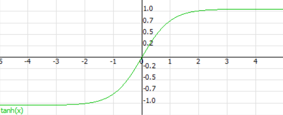
tanh

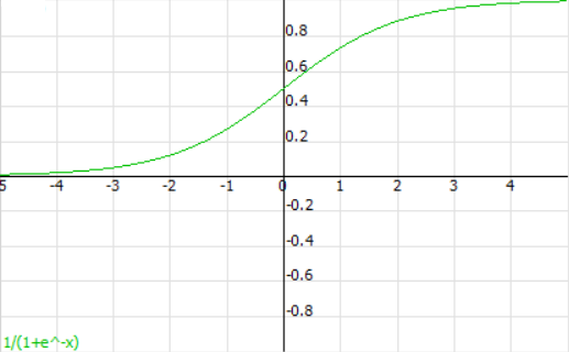
sigmoid

backward

void NeuralNetwork::backward(RowVector& output) {
    // calculate last layer errors
    *mErrors.back() = output - *mNeurons.back();

    // calculate hidden layers' errors (vector multiplication)
    for (size_t i = mErrors.size() - 2; i > 0; i--)
        *mErrors[i] = *mErrors[i + 1] * mWeights[i]->transpose();

    // update weights
    size_t size = mWeights.size();
    for (size_t i = 0; i < size; i++)
        for (int col = 0, cols = (int)mWeights[i]->cols(); col < cols; col++)
            for (int row = 0; row < mWeights[i]->rows(); row++) {
                mWeights[i]->coeffRef(row, col) +=
                    mLearningRate *
                    mErrors[i + 1]->coeffRef(col) *
                    activationDerivative(mNeurons[i + 1]->coeffRef(col)) *
                    mNeurons[i]->coeffRef(row);
            }
}

The function is key of the Backpropagation algorithm. It takes output of last layer and propagates backward through network layers, calculates each layer errors, and update connections weights depending on the rule:
new weight = old weight + learingRate * next error * sigmoidDerivative(next neuron value)

double NeuralNetwork::activationDerivative(double x) {
    if (mActivation == TANH)
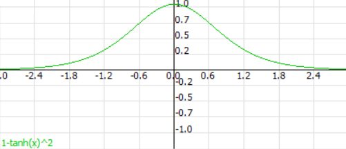
        return 1 - tanh(x) * tanh(x);
    if (mActivation == SIGMOID)
        return x * (1.0 - x);
    return 0;
}

tanh derivative

sigmoid derivative

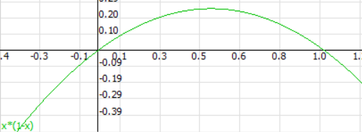
Note: The curve of sigmoidDerivative has a big significance. As its input ranges from 0 to 1 (neuron value), there are the three possible cases:

1. neuron value near 0, so weight value doesn't need support.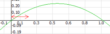

   

2. neuron value near 0.5, so weight value needs a slight change.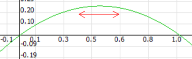

   

3. neuron value near 1, so weight value doesn't need support.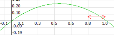

   

train

void NeuralNetwork::train(RowVector& input, RowVector& output) {
	forward(input);
	backward(output);
}

The function propagates input in forward direction, then propagates backward with the resultant output to adjust connections weight.

test

void NeuralNetwork::test(RowVector& input, RowVector& output) {
	forward(input);
	// calculate last layer errors
	*mErrors.back() = output - *mNeurons.back();
}

The function propagates input in forward direction, then calculates error between resultant output and desired output.

evaluate

There are various ways to evaluate the performance of neural network model, such as Confusion matrix, Accuracy, Precision, Recall, and F1 score. I have added “Confusion Matrix” calculation to the code through the evaluate function call after each testing call.

void NeuralNetwork::evaluate(RowVector& output) {
	double desired = 0, actual = 0;
	mConfusion->coeffRef(
		vote(output, desired),
		vote(*mNeurons.back(), actual)
	)++;
}

This function simply fill the right cell in the confusion matrix depending on the match between the actual and desired output.

After the hole testing the confusion matrix can be used to calculate Precision, Recall, and F1 score.

void NeuralNetwork::confusionMatrix(RowVector*& precision, RowVector*& recall) {
	int rows = (int)mConfusion->rows();
	int cols = (int)mConfusion->cols();
		
	precision = new RowVector(cols);
	for (int col = 0; col < cols; col++) {
		double colSum = 0;
		for (int row = 0; row < rows; row++)
			colSum += mConfusion->coeffRef(row, col);
		precision->coeffRef(col) = mConfusion->coeffRef(col, col) / colSum;
	}
	
	recall = new RowVector(rows);
	for (int row = 0; row < rows; row++) {
		double rowSum = 0;
		for (int col = 0; col < cols; col++)
			rowSum += mConfusion->coeffRef(row, col);
		recall->coeffRef(row) = mConfusion->coeffRef(row, row) / rowSum;
	}
	
	...
}

This calclation will be clear in the second Usecase Handwritten Digits Recognition

Use Cases

Simple Counter

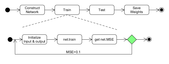
Neural network takes an input in binary (3 bits) and generates an output equals to input + 1. Then output is taken back as an input to the network. If input number equals to 7 (111 in binary) output should be 0. Network is trained using backpropagation algorithm to adjust network's connections weights. Training process takes about 2 minutes to minimize error between desired output and actual network output.

Input	Output
0 0 0	0 0 1
0 0 1	0 1 0
0 1 0	0 1 1
0 1 1	1 0 0
1 0 0	1 0 1
1 0 1	1 1 0
1 1 0	1 1 1
1 1 1	0 0 0

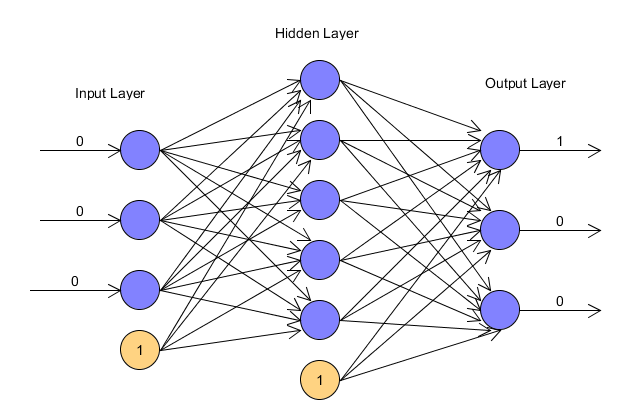
Simply, construct NeuralNetwork class with the required architecture and learningRate.

NeuralNetwork net({ 3, 5, 3 }, 0.05, NeuralNetwork::Activation::TANH);

3 neurons in input layer, 5 neurons in hidden layer, and 3 neurons in output layer.
0.05 learning rate.

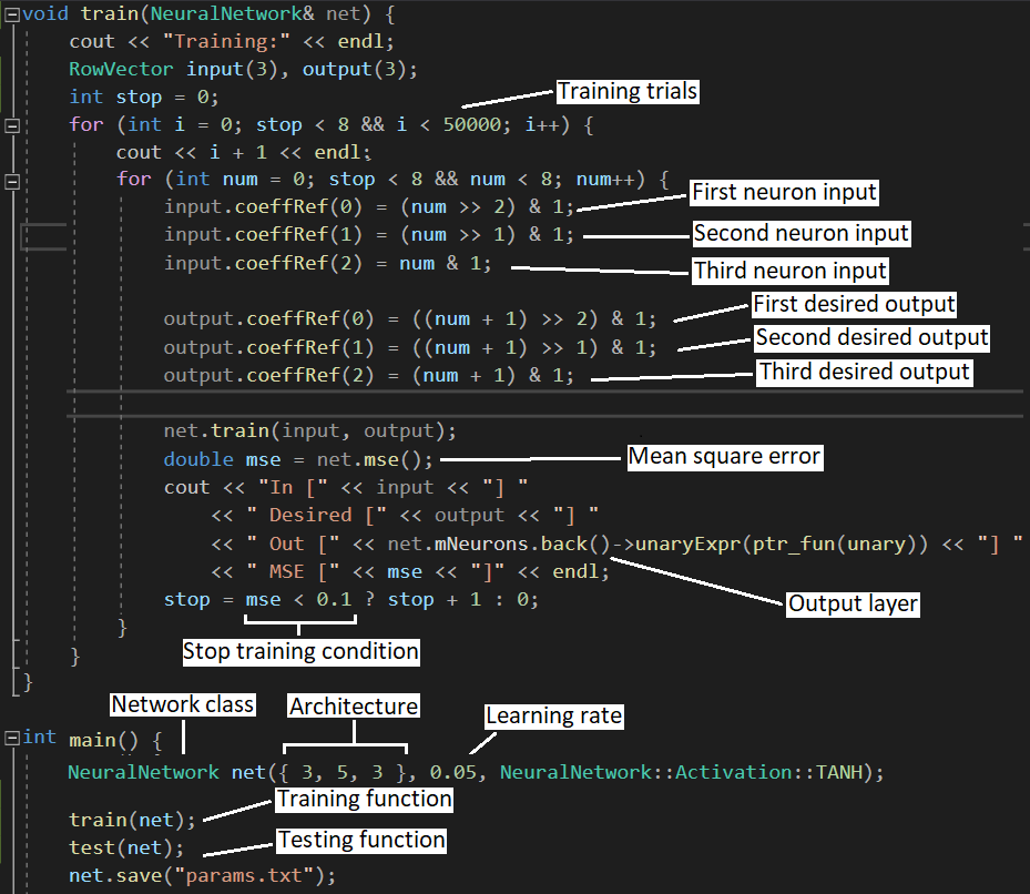
The following figure describes full training process for the network with 50,000 trials.

Train Network

void train(NeuralNetwork& net) {
	cout << "Training:" << endl;
    RowVector input(3), output(3);
	int stop = 0;
	for (int i = 0; stop < 8 && i < 50000; i++) {
		cout << i + 1 << endl;
		for (int num = 0; stop < 8 && num < 8; num++) {
			input.coeffRef(0) = (num >> 2) & 1;
			input.coeffRef(1) = (num >> 1) & 1;
			input.coeffRef(2) = num & 1;

			output.coeffRef(0) = ((num + 1) >> 2) & 1;
			output.coeffRef(1) = ((num + 1) >> 1) & 1;
			output.coeffRef(2) = (num + 1) & 1;

			net.train(input, output);
			double mse = net.mse();
			cout << "In [" << input << "] "
				<< " Desired [" << output << "] "
				<< " Out [" << net.mNeurons.back()->unaryExpr(ptr_fun(unary)) << "] "
				<< " MSE [" << mse << "]" << endl;
			stop = mse < 0.1 ? stop + 1 : 0;
		}
	}
}

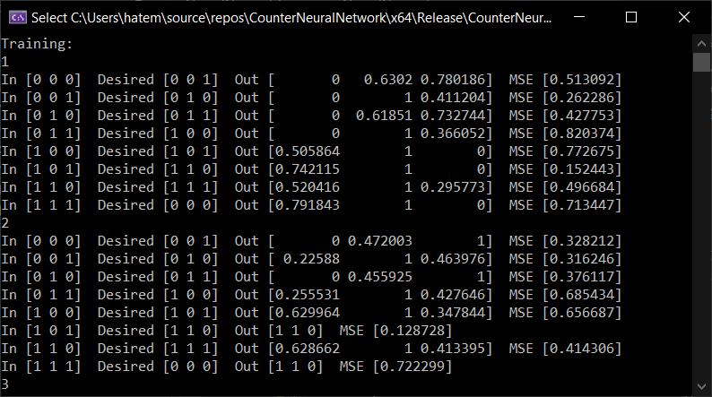
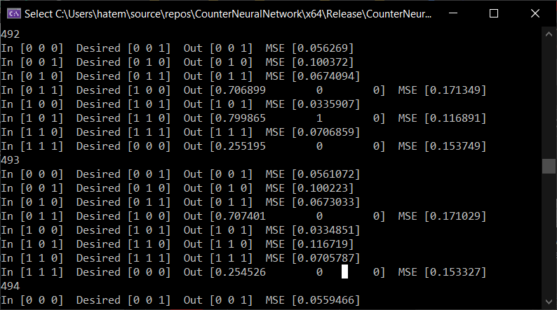
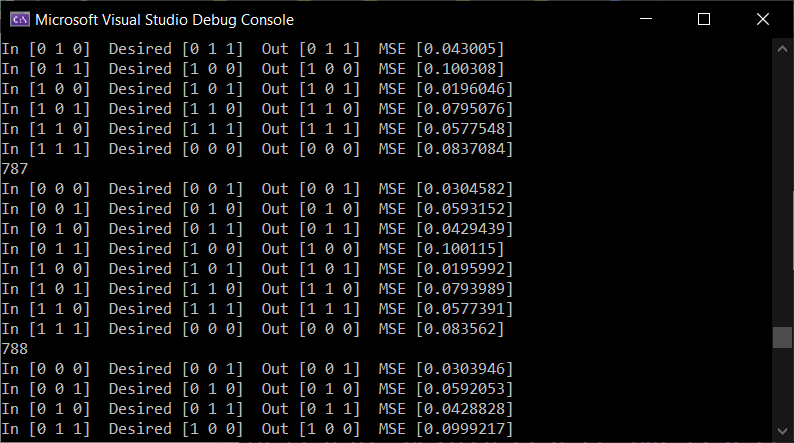
The function takes a network with an architecture { 3, 5, 3 } and does 50000x8 training call till it reaches acceptable error margin. After each training call, it displays input, output, and desired output.

1. In the first stages of training, the MSE (mean square error) is large, and output is so far from desired output.

   

2. After many rounds of training, the MSE decreased, and output came closer to desired output.

   

3. Finally, after 788 rounds, the MSE became less than 0.1 and the output was close to desired output.

   

Test Network

void test(NeuralNetwork& net) {
	cout << "Testing:" << endl;

    RowVector input(3), output(3);
	for (int num = 0; num < 8; num++) {
		input.coeffRef(0) = (num >> 2) & 1;
		input.coeffRef(1) = (num >> 1) & 1;
		input.coeffRef(2) = num & 1;

		output.coeffRef(0) = ((num + 1) >> 2) & 1;
		output.coeffRef(1) = ((num + 1) >> 1) & 1;
		output.coeffRef(2) = (num + 1) & 1;

		net.test(input, output);

		double mse = net.mse();
		cout << "In [" << input << "] "
			<< " Desired [" << output << "] "
			<< " Out [" << net.mNeurons.back()->unaryExpr(ptr_fun(unary)) << "] "
			<< " MSE [" << mse << "]" << endl;
	}
}

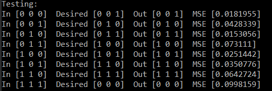
This function tests some inputs with the pre-trained network. It prints resultant output and MSE.

Save Network

int main() {
    NeuralNetwork net({ 3, 5, 3 }, 0.05);
    RowVector input(3), output(3);
	
    train(net, input, output);
    test(net, input, output);
    net.save("params.txt"); // Save architecture and weights
	
    return 0;
}

After training and testing network, we can save network structure in a file to be loaded later for network usage without retraining.

For our case, resultant file contains:

learningRate: 0.05
architecture: 3,5,3
activation: 0
weights: 
  -1.34013   0.811848   0.314629    1.85447  -0.343212   0.151176
   0.98971  -0.684254    1.20649   0.260128   -6.50245   -2.31706
  0.702027   -3.15824   -0.80735    1.07841   -2.57619   -2.17761
   0.13025    3.17894   0.594173   -3.18092 -0.0574412   -2.39394,
 -2.67379  0.467493  0.403606
 -1.22918   1.67581   1.60877
   1.1605  -1.95284  0.942444
 -1.92978 -0.704029  -1.12284
 -1.34765   -2.8206   1.44205
-0.996246  -1.52939  0.205469

The first line in weights section represents weights between first neuron in input layer and all neurons of next layer:

-1.34013   0.811848   0.314629    1.85447  -0.343212   0.151176

The second line in weights section represents weights between second neuron in input layer and all neurons of next layer:

0.98971  -0.684254    1.20649   0.260128   -6.50245   -2.31706

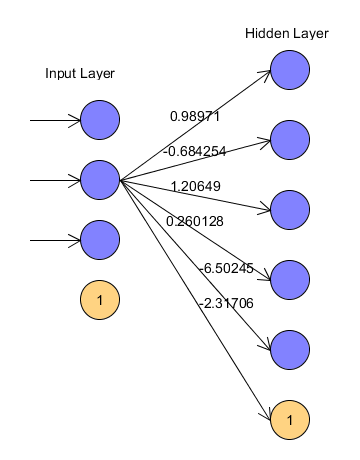
and, so on ...

Handwritten Digits Recognition

Handwritten recognition is one of the most successful application for Artificial Neural Network. It is the "Hello world" application for Neural Network study. In the previous use case, I use a shallow neural network, which has three layers of neurons that process inputs and generate outputs. Shallow neural networks can handle equally complex problems. But, in Handwritten Recognition, we need more accuracy and nonlinearity. Therefore, I have to use Deep Neural Network (DNN). DNN has two or more hidden layers of neurons that process inputs.

Network Architecture

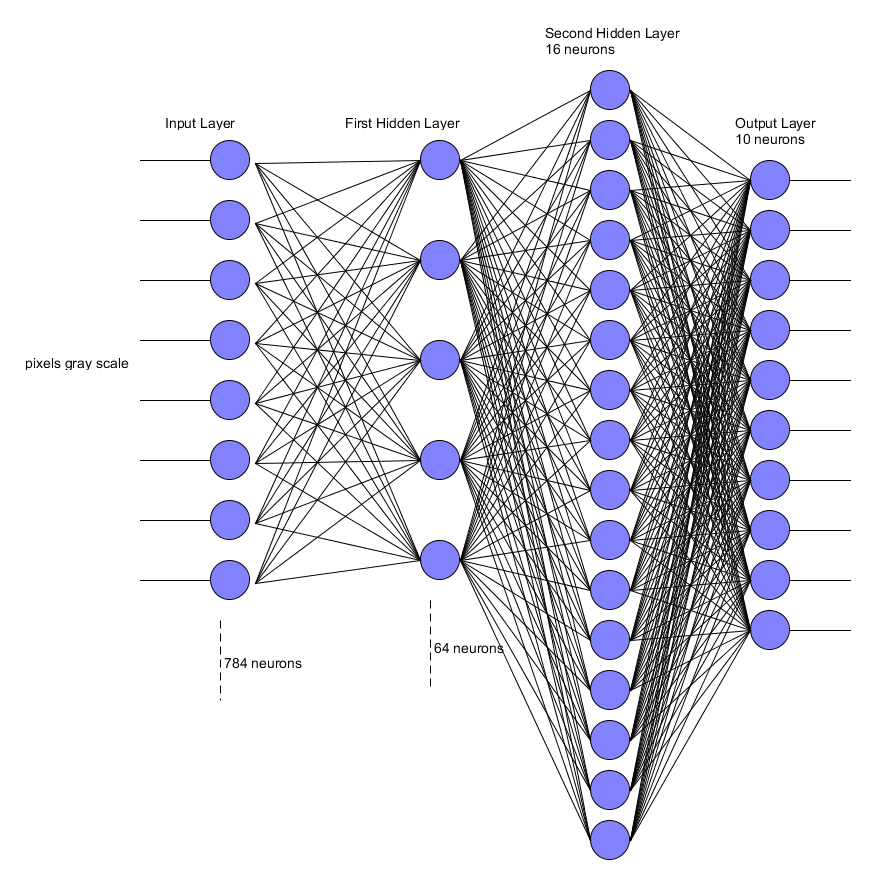
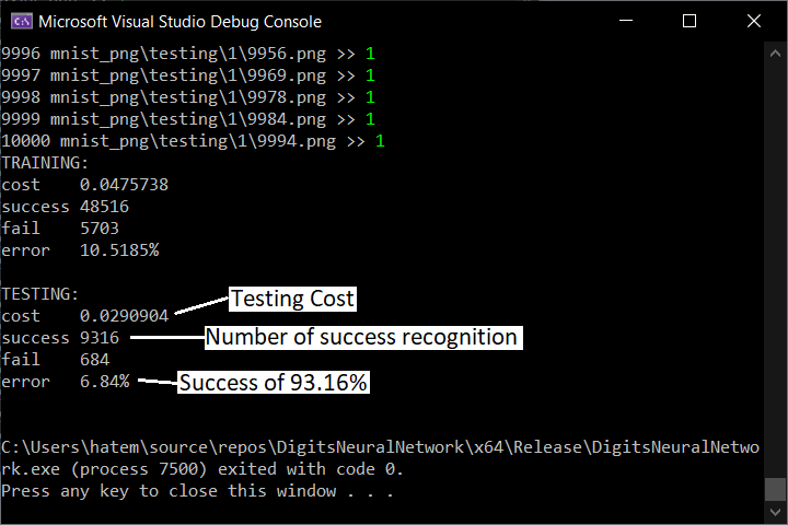
Using a network architecture {784, 64, 16, 10} (input - two hidden layers - output), I have achieved a success of 93.16%.

Activity Diagram

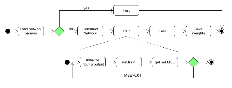
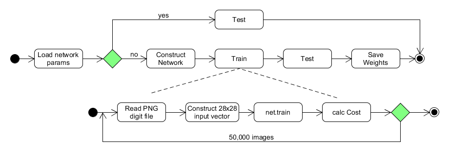
The following figure illustrates activity diagram of the whole process.

Used Libraries

This project uses:

• MNIST dataset for network training and testing. You have to download MNIST dataset files and put them in project execution path.
• libpng library for PNG files reading. You can download libpng16 (lib - h) files and put it in project build path.
• zlib library used internally by libpng16 to decompress images.

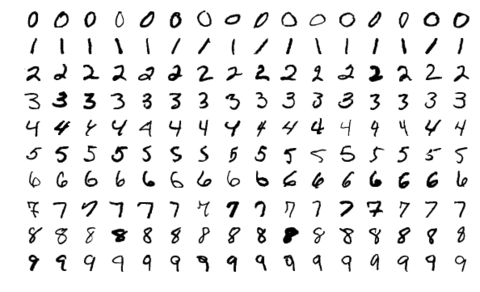
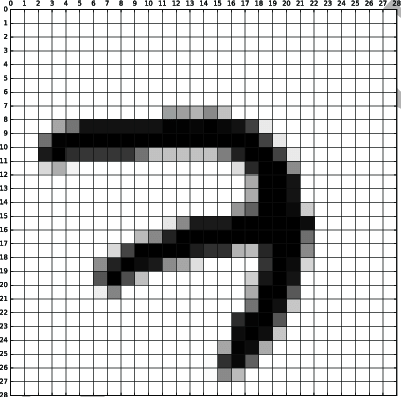
MNIST dataset contains 60,000 training images of handwritten digits from zero to nine and 10,000 images for testing. So, the MNIST dataset has 10 different classes. The handwritten digits images are represented as a 28×28 matrix where each cell contains grayscale pixel value (0 to 1).

Training and Testing

During training and testing, digit is read from its PNG file and converted from 28x28 image to a 784 double value of gray scale. This vector represented the input to the input layer of the neural network.

void readPng(const char* filepath, RowVector*& data) {
	pngwriter image;
	image.readfromfile(filepath);
	int width = image.getwidth(); // 28 
	int height = image.getheight(); // 28
	data = new RowVector(width * height); // 784

	for (int y = 0; y < height; y++)
		for (int x = 0; x < width; x++)
			data->coeffRef(0, y * width + x) = image.dread(x, y);
}

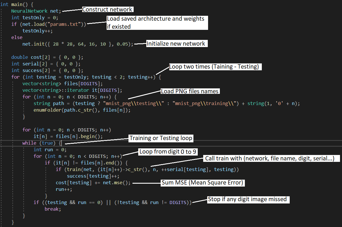
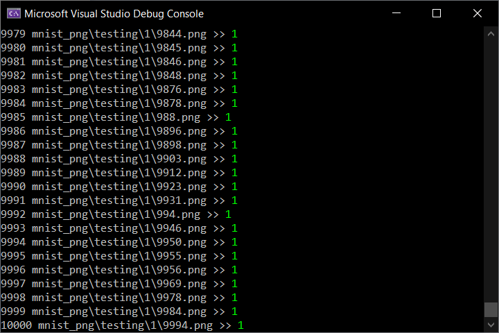
The following figure describes full training and testing processes for the network with 60,000 images (50,000 training - 10,000 testing).

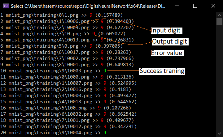
1. In the first stages of training, error is large and the output is so far from the desired output.

   

2. After many rounds of training, the MSE decreased and the output came closer to the desired output.

   

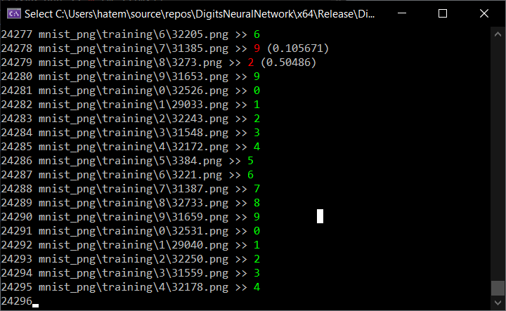
3. After testing 10000 images:

   

4. Display Training and Testing Cost and error percentage:

   

Save Network

int main() {
    .......
	if (!testOnly)
		net.save("params.txt");
	
    return 0;
}  

After training and testing network, we can save network structure in a file to be loaded later for network usage without retraining. If you are going to retrain, you have to delete the file "params.txt" from build path.
For our case resultant file contains:

learningRate: 0.05
architecture: 784,64,16,10
activation: 1
weights: 
   -0.997497    -0.307718   -0.0558184     0.124485    -0.188635     0.557909     0.242286 
   -0.898618    -0.942442     0.355693     0.284951     0.100192     0.724357    -0.998474 
    0.763909    -0.127537     0.893246    -0.956969    -0.492111    -0.775506    -0.603442 
   -0.907712    -0.987793   -0.0556963    -0.510117     0.450484     0.644276     0.951292 
    0.105869     -0.76458     0.586596     0.480819     0.253029    -0.672964    -0.418134 
    0.117222     0.121494     0.439985    -0.459639    -0.514145     0.458296     0.639027 
   -0.926817    -0.581164     0.774529    -0.392315    -0.985656     0.405133   -0.0527665
   -0.0163884  -0.00704978     0.138768      -0.2219    -0.927671    -0.880856     0.977355
   -0.927854     0.253273    -0.154149    -0.877621     0.797845     0.388653    0.0682699
    0.3361    -0.108066
    0.127171    -0.962889      0.39848    -0.457381     0.470931    -0.574816    -0.820429
   -0.851558    -0.925108     0.224769     0.575488     0.975402    -0.688955      0.78692 
    0.0274972    -0.218848    -0.790765     0.708121     0.144139    -0.574694     0.749809
    0.781732     0.362285    -0.662099    -0.903134     0.375225     0.581286    -0.679678 
    0.0863369     0.295511    -0.418195     0.241249    -0.720573    -0.794733    0.0434278 
   -0.81109     0.895749     0.652699     0.970824     0.643422   -0.0625935     0.776421
   -0.656117      0.23075     -0.18247    -0.250649    -0.197546     0.621632     0.804376 
   -0.976745     0.178747     0.137059    -0.404828    -0.564013    -0.309915    -0.376385  
   -0.66924     0.245216      -0.3961     0.160741     0.364788     0.150121    -0.811396 
   -0.837397    -0.901669    
....

Evaluation

After testing the network we can calculate evaluation items Precision, Recall, and F1 score from the Confusion Matrix.

Precision is the ratio between correct recognition (true positive) to predicted digit.

Precision = (0.95+0.97+0.95+0.95+0.92+0.93+0.96+0.95+0.94+0.89)/10 = 94%

Recall is the ratio between correct recognition (true positive) to actual digit.

Recall = (0.98+0.98+0.93+0.93+0.92+0.94+0.93+0.94+0.92+0.92)/10 = 94%

void evaluate(NeuralNetwork& net) {
	RowVector* precision, * recall;
	net.confusionMatrix(precision, recall);

	double precisionVal = precision->sum() / precision->cols();
	double recallVal = recall->sum() / recall->cols();
	double f1score = 2 * precisionVal * recallVal / (precisionVal + recallVal);

	cout << "Confusion matrix:" << endl;
	cout << *net.mConfusion << endl;
	cout << "Precision: " << (int)(precisionVal * 100) << '%' << endl;
	cout << *precision << endl;
	cout << "Recall: " << (int)(recallVal * 100) << '%' << endl;
	cout << *recall << endl;
	cout << "F1 score: " << (int)(f1score * 100) << '%' << endl;
	delete precision;
	delete recall;
}

The resultant values are like that:

Confusion matrix:
   98.6735   0.102041          0   0.102041          0   0.204082   0.306122   0.306122   0.306122          0
5.659e-313    98.2379   0.264317   0.176211          0          0   0.264317   0.176211   0.792952  0.0881057
   1.06589   0.290698    93.5078   0.387597    1.45349   0.290698   0.484496    1.16279   0.968992   0.387597
         0    0.29703    1.18812    93.5644  0.0990099    1.48515    0.29703   0.990099   0.891089    1.18812
  0.101833          0   0.407332   0.101833    92.9735          0   0.916497   0.203666          0    5.29532
   0.44843   0.112108   0.112108    2.01794   0.336323    94.2825    0.44843   0.560538    1.00897   0.672646
   1.46138   0.313152   0.417537          0    1.04384    2.71399    93.6326   0.104384   0.313152          0
         0    1.07004    1.16732   0.194553   0.583658   0.194553          0    94.5525  0.0972763    2.14008
  0.616016   0.513347   0.616016    1.12936    1.12936   0.718686   0.821355   0.821355    92.4025    1.23203
   0.99108   0.396432          0   0.891972    3.07235   0.396432   0.099108   0.693756    0.49554    92.9633
Precision: 94%
 0.95459 0.972949 0.958292 0.951662 0.922222 0.934444 0.961415 0.951076 0.948367 0.895893
Recall: 94%
0.986735 0.982379 0.935078 0.935644 0.929735 0.942825 0.936326 0.945525 0.924025 0.929633
F1 score: 94%

We can visualize the confusion matrix in the following table:

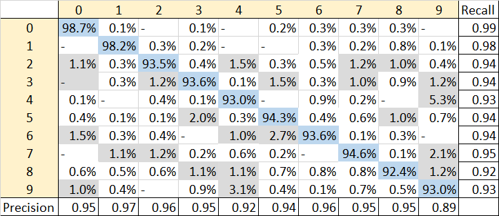
This table shows how often the model classified each digit correctly in blue, and which digits were most often confused for that label in gray.

History

• 24^th January, 2021: Initial post
• 7^th March, 2021: Evaluate model with Confusion Matrix

• NeuralNetwork 클래스 소스 파일 다운로드 - 3KB
• CounterNeuralNetwork 소스 파일 다운로드 - 6KB
• DigitsNeuralNetwork 소스 파일 다운로드 - 117KB

NeuralNetwork_src.zip CounterNeuralNetwork_src.zip DigitsNeuralNetwork_src.zip

내용물

• 배경
• 소개
• 신경망 클래스
  • 앞으로
  • 뒤로
  • 기차
  • 시험
  • 평가하다
• 사용 사례
  • 단순 카운터
    • 열차 네트워크
    • 테스트 네트워크
    • 네트워크 저장
  • 필기체 숫자 인식
    • 네트워크 아키텍처
    • 활동 다이어그램
    • 중고 라이브러리
    • 훈련 및 테스트
    • 네트워크 저장
    • 평가
• 역사

배경

이 글은 (ANN) 인공신경망의 과학적 측면을 설명하기 위한 것이 아닙니다. 역전파 알고리즘 의 수학적 계산이 복잡하지 않은 간단한 C++ 클래스를 제공합니다 . ANN에 대한 좋은 경험이 있으면 다음 섹션으로 건너뛰어도 됩니다. 그렇지 않으면 ANN에 대한 매우 유용한 리소스를 수정해도 됩니다. 코드 사용을 최대한 용이하게 하기 위해 두 가지 사용 사례를 제공했습니다.

• 신경망 소개
• 신경망 애플리케이션
• 역전파 수학
• 역전파 알고리즘

소개

오늘날 (ANN) 인공 신경망은 산업이든 가정이든 삶의 여러 영역에서 지배적이 되었습니다. ANN을 사용하면 기계가 인간의 두뇌를 학습하고 시뮬레이션하여 패턴을 인식하고 예측을 하며 모든 비즈니스 부문의 문제를 해결할 수 있습니다. 우리가 매일 사용하는 스마트폰과 컴퓨터는 일부 애플리케이션에서 ANN을 사용하고 있습니다. 예를 들어 스마트폰과 컴퓨터의 지문인식과 얼굴인식 잠금해제 서비스는 ANN을 사용합니다. 자필 서명 확인은 ANN을 사용합니다. 역전파 알고리즘을 처리하는 인공 신경망 C++ 클래스에 대한 간단한 구현을 작성했습니다. 코드는 Matrices의 수학을 처리하기 위해 Eigen 오픈 소스 템플릿에 의존합니다. 코드를 최대한 간단하고 빠르게 만들었습니다.

NeuralNetwork 클래스

NeuralNetwork다음 구조를 가진 간단한 C++ 클래스입니다.

코드는 템플릿 라이브러리 RowVectorXd를 MatrixXd사용 합니다 Eigen. 주요 기능은 "train"입력 "test"과 원하는 출력을 RowVector형식으로 취합니다. 둘 다 벡터 곱셈을"forward" 사용하는 함수를 호출합니다 .

앞으로

void NeuralNetwork::forward(RowVector& input) {
     // 첫 번째 레이어 입력 설정
     mNeurons.front()- > block( 0 , 0 , 1 , input.size()) = input; // 순방향 전파(벡터 곱셈)
 for ( unsigned int i = 1 ; i < mArchitecture.size(); i++) {
         // 바이어스이므로 마지막 뉴런에 값을 복사합니다
         mNeurons[i]- > block( 0 , 0 , 1 , mArchitecture[i]) = 
            (*mNeurons[i - 1 ] * *mWeights[i - 1 ]).block( 0 , 0 , 1 , mArchitecture[i]);
        for ( int col = 0 ; col < mArchitecture[i]; col++) 
            mNeurons[i]- > coeffRef(col) = 활성화(mNeurons[i]- > coeffRef(col)); 
    } 
}

         

이 함수는 네트워크 계층을 통해 입력을 전파하여 마지막 계층에서 출력을 얻습니다. 은닉층의 각 뉴런은 먼저 입력의 가중치 합을 계산합니다. 그런 다음 이 합계에 활성화 함수(세그모이드)를 적용하여 출력을 도출합니다. 이 함수는 뉴런 값에만 영향을 미칩니다. 연결 가중치나 오류에는 영향을 주지 않습니다. 이 함수는 벡터 곱셈을 통해 이 합을 계산합니다 .

(*mNeurons[i - 1 ] * *mWeights[i - 1 ])

그런 다음 결과 값이 함수를 통해 전달됩니다 activation.

double NeuralNetwork::activation( double x) {
     if (mActivation == TANH)
         return tanh(x);
    if (mActivation == SIGMOID)
         1 을 반환합니다  . 0 / ( 1 . 0 + exp(-x));
    0을 반환합니다 ; 
} 

탄

시그모이드

뒤로

void NeuralNetwork::backward(RowVector& 출력) {
     // 마지막 레이어 오류 계산
     *mErrors.back() = 출력 - *mNeurons.back(); // 숨겨진 레이어의 오류(벡터 곱셈)를 계산합니다
 for ( size_t i = mErrors.size() - 2 ; i > 0 ; i--) 
        *mErrors[i] = *mErrors[i + 1 ] * mWeights[i] - > 전치(); // 가중치 업데이트
 size_t size = mWeights.size();
    for ( size_t i = 0 ; i < size; i++)
         for ( int col = 0 , cols = ( int )mWeights[i]- > cols(); col < cols; col++)
             for ( int row = 0 ; row < mWeights[i]- > 행(); row++) { 
                mWeights[i]- > coeffRef(row, col) += 
                    mLearningRate * 
                    mErrors[i + 1 ]- > coeffRef(col) * 
                    activateDerivative(mNeurons[i + 1 ] - > coeffRef(col)) * 
                    mNeurons[i]- > coeffRef(row); 
            } 
}

         

        

이 기능은 역전파 알고리즘의 핵심입니다. 마지막 레이어의 출력을 가져와서 네트워크 레이어를 통해 역방향으로 전파하고, 각 레이어 오류를 계산하고, 규칙에 따라 연결 가중치를 업데이트합니다.
new weight = old weight + learingRate * next error * sigmoidDerivative(next neuron value)

double NeuralNetwork::activationDerivative( double x) {
     if (mActivation == TANH)
         return  1 - tanh(x) * tanh(x);
    if (mActivation == SIGMOID)
         return x * ( 1 . 0 - x);
    0을 반환합니다  ; 
}

탄 파생물

시그모이드 파생상품

참고 : 의 곡선은 sigmoidDerivative큰 의미를 갖습니다. 입력 범위는 0에서 1(뉴런 값)까지이므로 세 가지 경우가 가능합니다.

1. 근처의 뉴런 값 0이므로 가중치 값에는 지원이 필요하지 않습니다.

   

2. 근처에 뉴런 값이 있으므로 0.5가중치 값을 약간 변경해야 합니다.

   

3. 근처의 뉴런 값 1이므로 가중치 값에는 지원이 필요하지 않습니다.

   

기차

void NeuralNetwork::train(RowVector& 입력, RowVector& 출력) { 
	전달(입력); 
	뒤로(출력); 
}

이 함수는 입력을 순방향으로 전파한 다음 결과 출력으로 역방향으로 전파하여 연결 가중치를 조정합니다.

시험

void NeuralNetwork::test(RowVector& 입력, RowVector& 출력) { 
	전달(입력); // 마지막 레이어 오류 계산
 	*mErrors.back() = 출력 - *mNeurons.back(); 
}
	

이 함수는 입력을 순방향으로 전파한 다음 결과 출력과 원하는 출력 간의 오류를 계산합니다.

평가하다

신경망 모델의 성능을 평가하는 방법에는 Confusion Matrix , Accuracy , Precision , Recall , F1 Score 등 다양한 방법이 있습니다 .  각 테스트 호출 후 평가 함수 호출 을 통해 코드에 "혼란 행렬" 계산을 추가했습니다 .

void NeuralNetwork::evaluate(RowVector& 출력) {
	 원하는 두 배 = 0 , 실제 = 0 ; 
	mConfusion- > coeffRef( 
		vote(output, Desired), 
		vote(*mNeurons.back(), Actual) 
	)++; 
}

이 함수는 실제 출력과 원하는 출력 간의 일치 여부에 따라 혼동 행렬의 올바른 셀을 채웁니다.

홀 테스트 후 혼동 행렬을 사용하여 정밀도, 재현율 및 F1 점수를 계산할 수 있습니다.

void NeuralNetwork::confusionMatrix(RowVector*& 정밀도, RowVector*& 회수) {
	 int 행 = ( int )mConfusion- > 행();
	int cols = ( int )mConfusion- > cols(); 
		
	정밀도 = new RowVector(cols);
	for ( int col = 0 ; col < cols; col++) {
		 double colSum = 0 ;
		for ( int row = 0 ; row < 행; row++) 
			colSum += mConfusion- > coeffRef(row, col); 
		정밀도- > coeffRef(col) = mConfusion- > coeffRef(col, col) / colSum; 
	} 
	
	회상 = new RowVector(행);
	for ( int 행 = 0 ; 행 < 행; row++) {
		 double rowSum = 0 ;
		for ( int col = 0 ; col < cols; col++) 
			rowSum += mConfusion- > coeffRef(row, col); 
		회상 - > coeffRef(행) = mConfusion- > coeffRef(행, 행) / rowSum; 
	} 
	
	... 
}

이 계산은 두 번째 사용 사례 필기 숫자 인식 에서 명확해집니다.

사용 사례

단순 카운터

신경망은 이진수(3비트)로 입력을 받아 입력 + 1과 동일한 출력을 생성합니다. 그런 다음 출력은 다시 네트워크의 입력으로 사용됩니다. 입력 수가 7(이진수로 111)이면 출력은 0이 되어야 합니다. 네트워크는 역전파 알고리즘을 사용하여 훈련되어 네트워크의 연결 가중치를 조정합니다. 원하는 출력과 실제 네트워크 출력 사이의 오류를 최소화하기 위해 훈련 과정은 약 2분 정도 소요됩니다.

입력	산출
0 0 0	0 0 1
0 0 1	0 1 0
0 1 0	0 1 1
0 1 1	1 0 0
1 0 0	1 0 1
1 0 1	1 1 0
1 1 0	1 1 1
1 1 1	0 0 0

간단하게 NeuralNetwork필요한 아키텍처와 learningRate.

NeuralNetwork net({ 3 , 5 , 3 }, 0 . 05 , NeuralNetwork::Activation::TANH);

입력 레이어에 3개의 뉴런, 은닉 레이어에 5개의 뉴런, 출력 레이어에 3개의 뉴런.
0.05 학습률.

다음 그림은 50,000번의 시도가 포함된 네트워크의 전체 훈련 프로세스를 설명합니다.

기차 네트워크

void train(NeuralNetwork& net) { 
	cout < <  " 훈련:"  < < endl; 
    RowVector 입력( 3 ), 출력( 3 );
	int 정지 = 0 ;
	for ( int i = 0 ; stop <  8 && i <  50000 ; i++) { 
		cout < < i + 1  < < endl;
		for ( int num = 0 ; stop <  8 && num <  8 ; num++) { 
			input.coeffRef( 0 ) = (num > >  2 ) & 1 ; 
			input.coeffRef( 1 ) = (num > >  1 ) & 1 ; 
			input.coeffRef( 2 ) = num & 1 ; 

			output.coeffRef( 0 ) = ((num + 1 ) > >  2 ) & 1 ; 
			output.coeffRef( 1 ) = ((num + 1 ) > >  1 ) & 1 ; 
			출력.coeffRef( 2 ) = (num + 1 ) & 1 ; 

			net.train(입력, 출력); 이중 mse = net.mse(); 
			cout < < " In [" < < input < < " ] " < < " 원하는 [" < < 출력 < < " ] " < < " Out [" < < net.mNeurons.back()- > unaryExpr(ptr_fun( 단항)) < < " ] " < < " MSE [" < < mse < < " ]" < < endl; 
			정지 = mse < 0 . 1 ? 정지 + 1 : 0 ; 
		} 
} 
	}
			   
				   
				   
				     

이 함수는 {3, 5, 3} 아키텍처의 네트워크를 사용하고 허용 가능한 오류 한계에 도달할 때까지 50000x8 훈련 호출을 수행합니다. 각 교육 호출 후에는 입력, 출력 및 원하는 출력이 표시됩니다.

1. 훈련의 첫 번째 단계에서는 MSE(평균 제곱 오차)가 크고 출력이 원하는 출력과 너무 다릅니다.

   

2. 여러 차례의 훈련 후에 MSE가 감소하고 출력이 원하는 출력에 가까워졌습니다.

   

3. 마지막으로 788라운드 후에 MSE는 0.1 미만이 되었고 출력은 원하는 출력에 가까워졌습니다.

   

테스트 네트워크

void test(NeuralNetwork& net) { 
	cout < <  " 테스트:"  < < endl; 

    RowVector 입력( 3 ), 출력( 3 );
	for ( int num = 0 ; num <  8 ; num++) { 
		input.coeffRef( 0 ) = (num > >  2 ) & 1 ; 
		input.coeffRef( 1 ) = (num > >  1 ) & 1 ; 
		input.coeffRef( 2 ) = num & 1 ; 

		output.coeffRef( 0 ) = ((num + 1 ) > >  2 ) & 1 ; 
		output.coeffRef( 1 ) = ((num + 1 ) > >  1 ) & 1 ; 
		출력.coeffRef( 2 ) = (num + 1 ) & 1 ; 

		net.test(입력, 출력); 이중 mse = net.mse(); 
		cout < < " In [" < < input < < " ] " < < " 원하는 [" < < 출력 < < " ] " < < " Out [" < < net.mNeurons.back()- > unaryExpr(ptr_fun( 단항)) < < " ] " < < " MSE [" < < mse < < " ]" < < endl; 
	} 
}

		   
			   
			   
			    

이 함수는 사전 훈련된 네트워크를 사용하여 일부 입력을 테스트합니다. 결과 출력과 MSE를 인쇄합니다.

네트워크 저장

int main() { 
    NeuralNetwork net({ 3 , 5 , 3 }, 0 . 05 ); 
    RowVector 입력( 3 ), 출력( 3 ); 
	
    train(순, 입력, 출력); 
    테스트(순, 입력, 출력); 
    net.save( " params.txt" ); // 아키텍처 및 가중치 저장
 	
    return  0 ; 
}

네트워크를 훈련하고 테스트한 후에는 재훈련 없이 네트워크 사용을 위해 나중에 로드할 수 있도록 네트워크 구조를 파일에 저장할 수 있습니다.

우리의 경우 결과 파일에는 다음이 포함됩니다.

학습률 : 0.05
 아키텍처 : 3,5,3
 활성화 : 0
 가중치 : 
  -1.34013 0.811848 0.314629 1.85447 -0.343212 0.151176 0.98971 
   -0.684254 1.20649 0.260128 -6.50245 -2.3 1706 0.702027 -3.15824 -0.80735 1.07841 -2.57619 
  -2.17761 0.13025 3.17894 0.594173 
   -3.18092 -0.0574412 - 2.39394, 
 -2.67379 0.467493 0.403606 
 -1.22918 1.67581 1.60877 
   1.1605 -1.95284 0.942444 -1.92978 -0.704029 -1.12284 -1.34765 
 -2.820 6 1.44205 
 -0.996246 
-1.52939 0.205469

가중치 섹션의 첫 번째 줄은 입력 레이어의 첫 번째 뉴런과 다음 레이어의 모든 뉴런 사이의 가중치를 나타냅니다.

-1.34013 0.811848 0.314629 1.85447 -0.343212 0.151176

가중치 섹션의 두 번째 줄은 입력 레이어의 두 번째 뉴런과 다음 레이어의 모든 뉴런 사이의 가중치를 나타냅니다.

0.98971 -0.684254 1.20649 0.260128 -6.50245 -2.31706

등등 ...

필기체 숫자 인식

필기 인식은 인공 신경망의 가장 성공적인 응용 프로그램 중 하나입니다. Hello world신경망 연구를 위한 " " 애플리케이션입니다 . 이전 사용 사례에서는 입력을 처리하고 출력을 생성하는 세 개의 뉴런 계층이 있는 얕은 신경망을 사용했습니다. 얕은 신경망은 똑같이 복잡한 문제를 처리할 수 있습니다. 그러나 필기 인식에서는 더 많은 정확성과 비선형성이 필요합니다. 그래서 DNN( Deep Neural Network )을 사용해야 합니다 . DNN에는 입력을 처리하는 두 개 이상의 숨겨진 뉴런 레이어가 있습니다.

네트워크 아키텍처

네트워크 아키텍처 {784, 64, 16, 10}(입력 - 2개의 숨겨진 레이어 - 출력)을 사용하여 93.16%의 성공을 달성했습니다.

활동 다이어그램

다음 그림은 전체 프로세스의 활동 다이어그램을 보여줍니다.

중고 라이브러리

이 프로젝트에서는 다음을 사용합니다.

• 네트워크 훈련 및 테스트를 위한 MNIST 데이터세트입니다 . MNIST 데이터 세트 파일을 다운로드하여 프로젝트 실행 경로에 넣어야 합니다 .
• PNG 파일 읽기를 위한 libpng 라이브러리입니다 . libpng16 (lib - h) 파일을 다운로드하여 프로젝트 빌드 경로에 넣을 수 있습니다 .
• 이미지 압축을 풀기 위해 libpng16에서 내부적으로 사용하는 zlib 라이브러리 입니다.

MNIST 데이터세트에는 0부터 9까지 손으로 쓴 숫자의 훈련 이미지 60,000개와 테스트용 이미지 10,000개가 포함되어 있습니다. 따라서 MNIST 데이터세트에는 10개의 서로 다른 클래스가 있습니다. 손으로 쓴 숫자 이미지는 각 셀에 회색조 픽셀 값(0~1)이 포함된 28×28 행렬로 표시됩니다.

훈련 및 테스트

훈련 및 테스트 중에 숫자는 PNG 파일에서 읽혀지고 28x28 이미지에서 784 이중 값의 회색조로 변환됩니다. 이 벡터는 신경망의 입력 레이어에 대한 입력을 나타냅니다.

void readPng( const  char * 파일 경로, RowVector*& 데이터) { 
	pngwriter 이미지; 
	image.readfromfile(파일 경로); int 너비 = image.getwidth(); // 28 
 int height = image.getheight(); // 28
 	data = new RowVector(너비 * 높이); // 784
 for ( int y = 0 ; y < height; y++)
		 for ( int x = 0 ; x < width; x++) 
			data- > coeffRef( 0 , y * width + x) = image.dread(x, y ); 
}
		
	

다음 그림은 60,000개의 이미지(50,000개 훈련 - 10,000개 테스트)가 있는 네트워크에 대한 전체 훈련 및 테스트 프로세스를 설명합니다.

1. 학습의 첫 번째 단계에서는 오류가 크고 출력이 원하는 출력과 너무 멀리 떨어져 있습니다.

   

2. 여러 차례의 훈련 후에 MSE가 감소하고 출력이 원하는 출력에 더 가까워졌습니다.

   

3. 10000개의 이미지를 테스트한 후:

   

4. 교육 및 테스트 비용 및 오류 비율 표시:

   

네트워크 저장

int main() { 
    ....... if (!testOnly) 
		net.save( " params.txt" ); 0을 반환합니다 ; 
}  
	
	
     

네트워크를 훈련하고 테스트한 후에는 재훈련 없이 네트워크 사용을 위해 나중에 로드할 수 있도록 네트워크 구조를 파일에 저장할 수 있습니다. 재학습하려면 빌드 경로에서 "params.txt" 파일을 삭제해야 합니다 .
우리의 경우 결과 파일에는 다음이 포함됩니다.

학습률 : 0.05
 아키텍처 : 784,64,16,10
 활성화 : 1
 가중치 : 
   -0.997497 -0.307718 -0.0558184 0.124485 -0.188635 0.557909 0.242286 -0.898618 -0.942442 0.355693 0.284951 0.100192 0.724357 -0.998474 0.763909 -0.127537 0.893246 
   -0.956969 -0.492111 
    -0.775506 -0.603442 
   -0.907712 -0.987793 -0.0556963 -0.510117 0.450484 0.644276 0.951292 
    0.105869 -0.76458 0.586596 0.480819 0.253029 -0.672964 -0.418134 
    0.117222 0.121494 0.439985 -0.459639 -0.514145 0.458296 0.639027 
   -0.926817 -0.581164 0.774529 -0.392315 -0.985656 0.405133 -0.0527665 
   -0.0163884 -0.00704978 0.138768 -0.2219 - 0.927671 -0.880856 0.977355 
   -0.927854 0.253273 -0.154149 -0.877621 0.797845 0.388653 0.0682699 
    0.3361 -0.108066 
    0.127171 -0.962889 0.39848 -0.457381 0.470931 -0.574816 -0.820429 
   -0.851558 -0.925108 0.224769 0.575488 0.975402 -0.688955 0.78692 
    0.0274972 -0.218848 -0.790765 0.708121 0.144139 -0.574694 0.749809 
    0.781732 0.362285 -0.662099 -0.903134 0.375225 0.581286 -0.679678 
    0.0863369 0.295511 -0.418195 0.241249 -0.720573 -0.794733 0.0434278 
   -0.81109 0.895749 0.652699 0.970824 0.643422 -0.0625935 0.776421 
   -0.656117 0.23075 -0.18247 -0.250649 -0.197546 0.621632 0.804376 
   -0.976745 0.178747 0.137059 -0.404828 -0.564013 -0.309915 -0.376385   
   -0.66924 0.245216 -0.3961 0.160741 0.364788 0.150121 -0.811396 
   -0.837397 -0.901669     
....

평가

네트워크를 테스트한 후 Confusion Matrix에서 평가 항목 Precision, Recall 및 F1 점수를 계산할 수 있습니다.

정밀도는 정확한 인식(진양성)과 예측된 숫자 간의 비율입니다.

정밀도 = ( 0 .95+0.97+0.95+0.95+0.92+0.93+0.96+0.95+0.94+ 0.89 )/10 = 94%

재현율은 올바른 인식(참양성)과 실제 숫자 간의 비율입니다.

재현율 = ( 0.98 +0.98+0.93+0.93+0.92+0.94+0.93+0.94+0.92+0.92 ) /10 = 94%

void 평가(NeuralNetwork& net) { 
	RowVector* 정밀도, * 재현율; 
	net.confusionMatrix(정밀도, 재현율); 배정 밀도Val = 정밀도- > sum() / 정밀도- > cols();
	double 회상Val = 회상- > sum() / 회상- > cols();
	double f1score = 2 * PrecisionVal * RecallVal / (PrecisionVal + RecallVal); 
	cout < < " 혼동행렬:" < < endl; 
	cout < < *net.mConfusion < < endl; 
	cout < < " 정밀도: " < < ( int )(precisionVal * 100 ) < < ' %' < < endl; 
	cout < < *정밀도 < < endl; 
	cout < < " 회상: " < < ( int )(recallVal * 100 ) < < ' %' < < endl; 
	cout < < *recall < < endl; 
	cout < < " F1 점수: " < < ( int )(f1score * 100 ) < < ' %' < < endl;
	정밀도
	 삭제 ; 회상 삭제 ; 
}

	
              

결과 값은 다음과 같습니다.

Confusion matrix:
   98.6735   0.102041          0   0.102041          0   0.204082   0.306122   0.306122   0.306122          0
5.659e-313    98.2379   0.264317   0.176211          0          0   0.264317   0.176211   0.792952  0.0881057
   1.06589   0.290698    93.5078   0.387597    1.45349   0.290698   0.484496    1.16279   0.968992   0.387597
         0    0.29703    1.18812    93.5644  0.0990099    1.48515    0.29703   0.990099   0.891089    1.18812
  0.101833          0   0.407332   0.101833    92.9735          0   0.916497   0.203666          0    5.29532
   0.44843   0.112108   0.112108    2.01794   0.336323    94.2825    0.44843   0.560538    1.00897   0.672646
   1.46138   0.313152   0.417537          0    1.04384    2.71399    93.6326   0.104384   0.313152          0
         0    1.07004    1.16732   0.194553   0.583658   0.194553          0    94.5525  0.0972763    2.14008
  0.616016   0.513347   0.616016    1.12936    1.12936   0.718686   0.821355   0.821355    92.4025    1.23203
   0.99108   0.396432          0   0.891972    3.07235   0.396432   0.099108   0.693756    0.49554    92.9633
Precision: 94%
 0.95459 0.972949 0.958292 0.951662 0.922222 0.934444 0.961415 0.951076 0.948367 0.895893
Recall: 94%
0.986735 0.982379 0.935078 0.935644 0.929735 0.942825 0.936326 0.945525 0.924025 0.929633
F1 score: 94%

다음 표에서 혼동 행렬을 시각화할 수 있습니다.

이 표는 모델이 각 숫자를 파란색으로 올바르게 분류한 빈도와 해당 레이블에 대해 가장 자주 혼동되는 숫자를 회색으로 보여줍니다.

역사

• 2021년 1월 24 ^일 : 최초 게시물
• 2021년 3월 7 ^일 : 혼동 ​​행렬을 사용하여 모델 평가