
- 전체
- Sample DB
- database modeling
- [표준 SQL] Standard SQL
- G-SQL
- 10-Min
- ORACLE
- MS SQLserver
- MySQL
- SQLite
- postgreSQL
- 데이터아키텍처전문가 - 국가공인자격
- 데이터 분석 전문가 [ADP]
- [국가공인] SQL 개발자/전문가
- NoSQL
- hadoop
- hadoop eco system
- big data (빅데이터)
- stat(통계) R 언어
- XML DB & XQuery
- spark
- DataBase Tool
- 데이터분석 & 데이터사이언스
- Engineer Quality Management
- [기계학습] machine learning
- 데이터 수집 및 전처리
- 국가기술자격 빅데이터분석기사
- 암호화폐 (비트코인, cryptocurrency, bitcoin)
[R 데이터 분석] Titanic: Machine Learning from Disaster (타이타닉 생존 예측)
Titanic: Machine Learning from Disaster (타이타닉 생존 예측)
Andrew Jang
10/2/2018
1. Predict survival on the Titanic
- Defining the problem statement
- Collecting the data
- Exploratory data analysis
- Feature engineering
- Modelling
- Testing
2. Defining the problem statement
Complete the analysis of what sorts of people were likely to survive.
In particular, we ask you to apply the tools of machine learning to predict which passengers survived the Titanic tragedy.

3. Collecting & Preprocessing the data
training data set and testing data set are given by Kaggle you can download from kaggle directly kaggle
3.1. Import library & Load dataset
suppressMessages(library(dplyr)) #edit
suppressMessages(library(readxl)) #excel load
suppressMessages(library(doBy))
suppressMessages(library(fmsb)) # radar chart
suppressMessages(library(ggplot2)) #visualization
suppressMessages(library(corrplot)) #correlation
suppressMessages(library(VIM)) #missing data detection
suppressMessages(library(DMwR)) #outlier detection
suppressMessages(library(corrplot)) #correlation plot
suppressMessages(library(PerformanceAnalytics)) #correlation chart
suppressMessages(library(RColorBrewer)) #decision tree fancy tree
suppressMessages(library(ipred)) # bagging
suppressMessages(library(adabag)) # adaptive boosting
suppressMessages(library(lme4)) #dummy function
suppressMessages(library(caret)) #standard
suppressMessages(library(class)) #KNN
suppressMessages(library(VennDiagram)) #VennDiagram
suppressMessages(library(neuralnet)) #ann
suppressMessages(library(e1071)) #SVM
suppressMessages(library(ROCR)) #ROC

suppressMessages(library(mctest))
suppressMessages(library(dummies))
suppressMessages(library(Information))


suppressMessages(library(rpart)) #decision tree
suppressMessages(library(C50)) # decision tree
suppressMessages(library(rattle)) #decision tree fancy tree
suppressMessages(library(rpart.plot)) #decision tree fancy tree
suppressMessages(library(randomForest)) # random forest
suppressMessages(library(pROC))
suppressMessages(library(gmodels)) # CrossTable
suppressMessages(library(glmnet)) # glmnet
suppressMessages(library(gbm)) # gbm

#library(tidyverse)
#library(gridExtra)
#library(MASS)

#library(boot)
#library(data.table)


train = read.csv('input/train.csv')
test = read.csv('input/test.csv')
3.2. Overview dataset
str(train)
## 'data.frame':    891 obs. of  12 variables:
##  $ PassengerId: int  1 2 3 4 5 6 7 8 9 10 ...
##  $ Survived   : int  0 1 1 1 0 0 0 0 1 1 ...
##  $ Pclass     : int  3 1 3 1 3 3 1 3 3 2 ...
##  $ Name       : Factor w/ 891 levels "Abbing, Mr. Anthony",..: 109 191 358 277 16 559 520 629 417 581 ...
##  $ Sex        : Factor w/ 2 levels "female","male": 2 1 1 1 2 2 2 2 1 1 ...
##  $ Age        : num  22 38 26 35 35 NA 54 2 27 14 ...
##  $ SibSp      : int  1 1 0 1 0 0 0 3 0 1 ...
##  $ Parch      : int  0 0 0 0 0 0 0 1 2 0 ...
##  $ Ticket     : Factor w/ 681 levels "110152","110413",..: 524 597 670 50 473 276 86 396 345 133 ...
##  $ Fare       : num  7.25 71.28 7.92 53.1 8.05 ...
##  $ Cabin      : Factor w/ 148 levels "","A10","A14",..: 1 83 1 57 1 1 131 1 1 1 ...
##  $ Embarked   : Factor w/ 4 levels "","C","Q","S": 4 2 4 4 4 3 4 4 4 2 ...
Total rows and columns
891개의 행과 12개의 변수가 훈련 데이터에 존재한다
3.3. Data Dictionary
- Survived:     0 = No, 1 = Yes
- pclass:   Ticket class    1 = 1st, 2 = 2nd, 3 = 3rd
- sibsp:    # of siblings / spouses aboard the Titanic
    - Siblings + Spouses : 0(혼자 탑승), 1(동승자 1인) ... n
- parch:    # of parents / children aboard the Titanic
    - Parents + Children
- ticket:   Ticket number
- cabin:    Cabin number
- embarked: Port of Embarkation C = Cherbourg, Q = Queenstown, S = Southampton
3.4. Reshape data type
train$Survived <- factor(train$Survived)
train$Pclass <- factor(train$Pclass)
3.5. Missing values
colSums(is.na(train))
## PassengerId    Survived      Pclass        Name         Sex         Age
##           0           0           0           0           0         177
##       SibSp       Parch      Ticket        Fare       Cabin    Embarked
##           0           0           0           0           0           0
colSums(is.na(test))
## PassengerId      Pclass        Name         Sex         Age       SibSp
##           0           0           0           0          86           0
##       Parch      Ticket        Fare       Cabin    Embarked
##           0           0           1           0           0
총 891개의 훈련 데이터 중에 "Age" 변수는 714개, "Cabin" 변수는 204개만 존재한다.

이렇게 유실된 정보(결측치)들을 머신러닝 모델에 넣으면 잘못된 정보를 야기한다.

모델링 전에 missing field는 feature engneering(preprocessing)을 통해 의미있는 정보로 바꿔주어야 한다.

테스트 데이터에도 비슷한 비율로 "Age" 변수와 "Cabin" 변수가 빠져 있다.
3.6. Outliers
summary(train)
##   PassengerId    Survived Pclass
##  Min.   :  1.0   0:549    1:216
##  1st Qu.:223.5   1:342    2:184
##  Median :446.0            3:491
##  Mean   :446.0
##  3rd Qu.:668.5
##  Max.   :891.0
##
##                                     Name         Sex           Age
##  Abbing, Mr. Anthony                  :  1   female:314   Min.   : 0.42
##  Abbott, Mr. Rossmore Edward          :  1   male  :577   1st Qu.:20.12
##  Abbott, Mrs. Stanton (Rosa Hunt)     :  1                Median :28.00
##  Abelson, Mr. Samuel                  :  1                Mean   :29.70
##  Abelson, Mrs. Samuel (Hannah Wizosky):  1                3rd Qu.:38.00
##  Adahl, Mr. Mauritz Nils Martin       :  1                Max.   :80.00
##  (Other)                              :885                NA's   :177
##      SibSp           Parch             Ticket         Fare
##  Min.   :0.000   Min.   :0.0000   1601    :  7   Min.   :  0.00
##  1st Qu.:0.000   1st Qu.:0.0000   347082  :  7   1st Qu.:  7.91
##  Median :0.000   Median :0.0000   CA. 2343:  7   Median : 14.45
##  Mean   :0.523   Mean   :0.3816   3101295 :  6   Mean   : 32.20
##  3rd Qu.:1.000   3rd Qu.:0.0000   347088  :  6   3rd Qu.: 31.00
##  Max.   :8.000   Max.   :6.0000   CA 2144 :  6   Max.   :512.33
##                                   (Other) :852
##          Cabin     Embarked
##             :687    :  2
##  B96 B98    :  4   C:168
##  C23 C25 C27:  4   Q: 77
##  G6         :  4   S:644
##  C22 C26    :  3
##  D          :  3
##  (Other)    :186
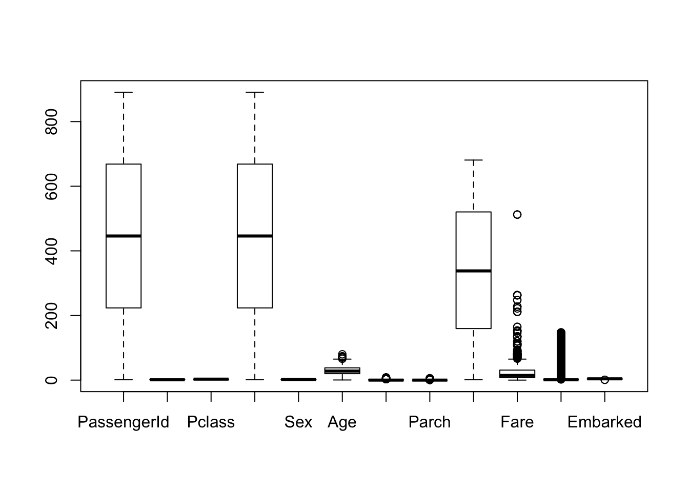
boxplot(train)
4. Exploratory data analysis
Printing first 5 rows of the train dataset.
head(train)
##   PassengerId Survived Pclass
## 1           1        0      3
## 2           2        1      1
## 3           3        1      3
## 4           4        1      1
## 5           5        0      3
## 6           6        0      3
##                                                  Name    Sex Age SibSp
## 1                             Braund, Mr. Owen Harris   male  22     1
## 2 Cumings, Mrs. John Bradley (Florence Briggs Thayer) female  38     1
## 3                              Heikkinen, Miss. Laina female  26     0
## 4        Futrelle, Mrs. Jacques Heath (Lily May Peel) female  35     1
## 5                            Allen, Mr. William Henry   male  35     0
## 6                                    Moran, Mr. James   male  NA     0
##   Parch           Ticket    Fare Cabin Embarked
## 1     0        A/5 21171  7.2500              S
## 2     0         PC 17599 71.2833   C85        C
## 3     0 STON/O2. 3101282  7.9250              S
## 4     0           113803 53.1000  C123        S
## 5     0           373450  8.0500              S
## 6     0           330877  8.4583              Q
Bar Chart for Categorical Features
- Pclass
- Sex
- SibSp ( # of siblings and spouse)
- Parch ( # of parents and children)
- Embarked
- Cabin
4.1. EDA 1 : Sex
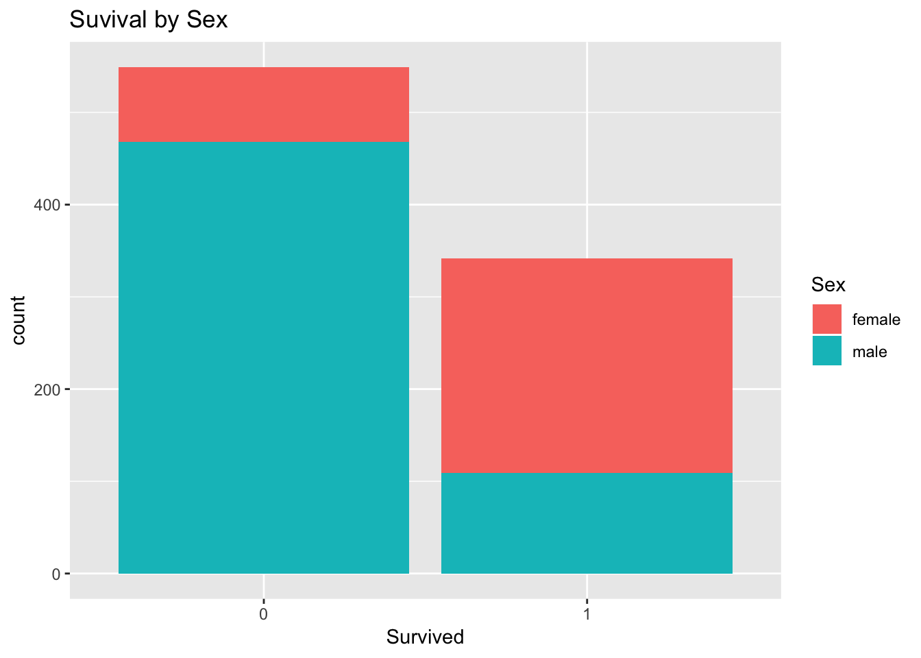
train %>% group_by(Survived, Sex) %>% summarise(freq = n())
## # A tibble: 4 x 3
## # Groups:   Survived [?]
##   Survived Sex     freq
##   <fct>    <fct>  <int>
## 1 0        female    81
## 2 0        male     468
## 3 1        female   233
## 4 1        male     109
ggplot(train, aes(x = Survived, fill=Sex))+geom_bar()+
  ggtitle("Suvival by Sex")
Summary 1
여자들은 남자보다 살아남을 확률이 상대적으로 높다는 것을 알 수 있다.
| 남자 | 여자 | |
|---|---|---|
| Prob. | 생존<사망 | 생존>사망 |
4.2. EDA 2 : Pclass
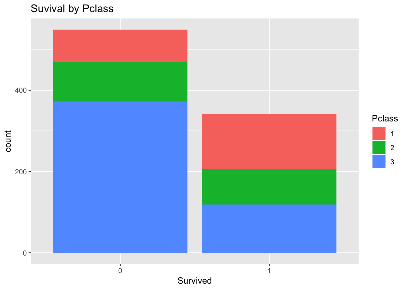
train %>% group_by(Survived, Pclass) %>% summarise(freq = n())
## # A tibble: 6 x 3
## # Groups:   Survived [?]
##   Survived Pclass  freq
##   <fct>    <fct>  <int>
## 1 0        1         80
## 2 0        2         97
## 3 0        3        372
## 4 1        1        136
## 5 1        2         87
## 6 1        3        119
ggplot(train, aes(x = Survived, fill=Pclass))+geom_bar()+
  ggtitle("Suvival by Pclass")
Summary 2
1등급은 다른 등급에 비해 살아남을 확률이 조금 더 높고, 3등급은 다른 등급에 비해 죽을 확률이 높다.
Pclass가 survived에 중요한 영향을 끼치는 변수라는 것을 알 수 있다.
| 1등급 | 2등급 | 3등급 | |
|---|---|---|---|
| Prob. | 생존>사망 | 생존>=사망 | 생존<사망 |
4.3. EDA 3 : SibSp
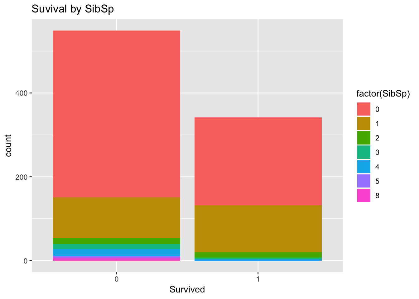
train %>% group_by(Survived, SibSp) %>% summarise(freq = n())
## # A tibble: 12 x 3
## # Groups:   Survived [?]
##    Survived SibSp  freq
##    <fct>    <int> <int>
##  1 0            0   398
##  2 0            1    97
##  3 0            2    15
##  4 0            3    12
##  5 0            4    15
##  6 0            5     5
##  7 0            8     7
##  8 1            0   210
##  9 1            1   112
## 10 1            2    13
## 11 1            3     4
## 12 1            4     3
ggplot(train, aes(x = Survived, fill=factor(SibSp)))+geom_bar()+
  ggtitle("Suvival by SibSp")
Summary 3
혼자 탄 승객이 사망자와 생존자 비율 중에서 가장 많지만 사망하는 사람의 비율이 압도적으로 많다(생존 23.57%, 사망 44.67%).
구성원을 기준으로 생존과 사망의 비율의 차이를 비교한 결과 유일하게 (본인을 포함한)2명의 생존율만 높았다.
그리고 가족의 수가 많아질수록 사망률이 늘어났다.
4.4. EDA 4 : Parch
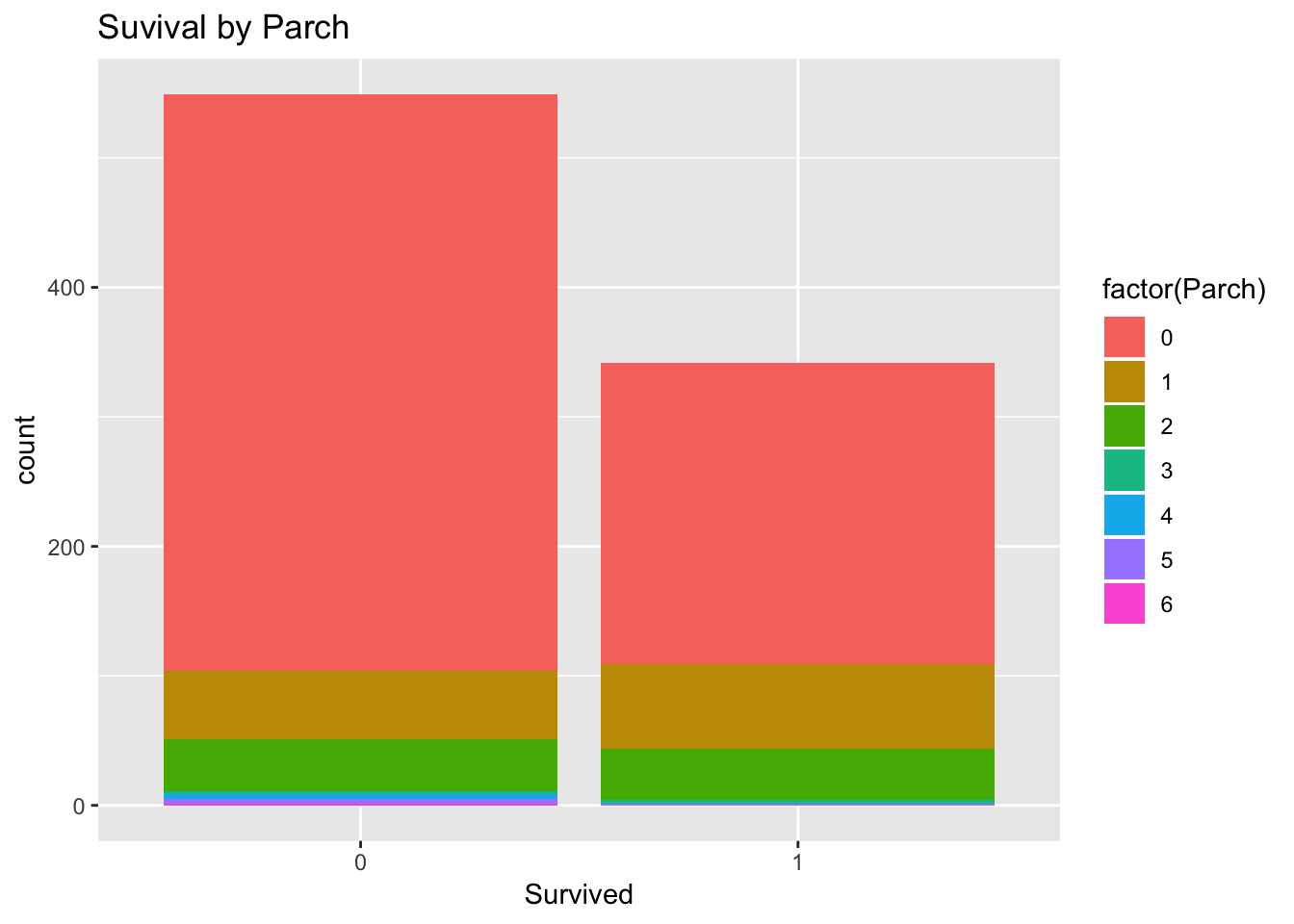
train %>% group_by(Survived, Parch) %>% summarise(freq = n())
## # A tibble: 12 x 3
## # Groups:   Survived [?]
##    Survived Parch  freq
##    <fct>    <int> <int>
##  1 0            0   445
##  2 0            1    53
##  3 0            2    40
##  4 0            3     2
##  5 0            4     4
##  6 0            5     4
##  7 0            6     1
##  8 1            0   233
##  9 1            1    65
## 10 1            2    40
## 11 1            3     3
## 12 1            5     1
ggplot(train, aes(x = Survived, fill=factor(Parch)))+geom_bar()+
  ggtitle("Suvival by Parch")
Summary 4
부모님이나 아이들과 동승했을 경우, 조금 더 많이 살았으나, 혼자 탄 승객은 많이 죽었다.
| 혼자 | 동승 | |
|---|---|---|
| Prob. | 생존<사망 | 생존>사망 |
4.5. EDA 5 : Embarked
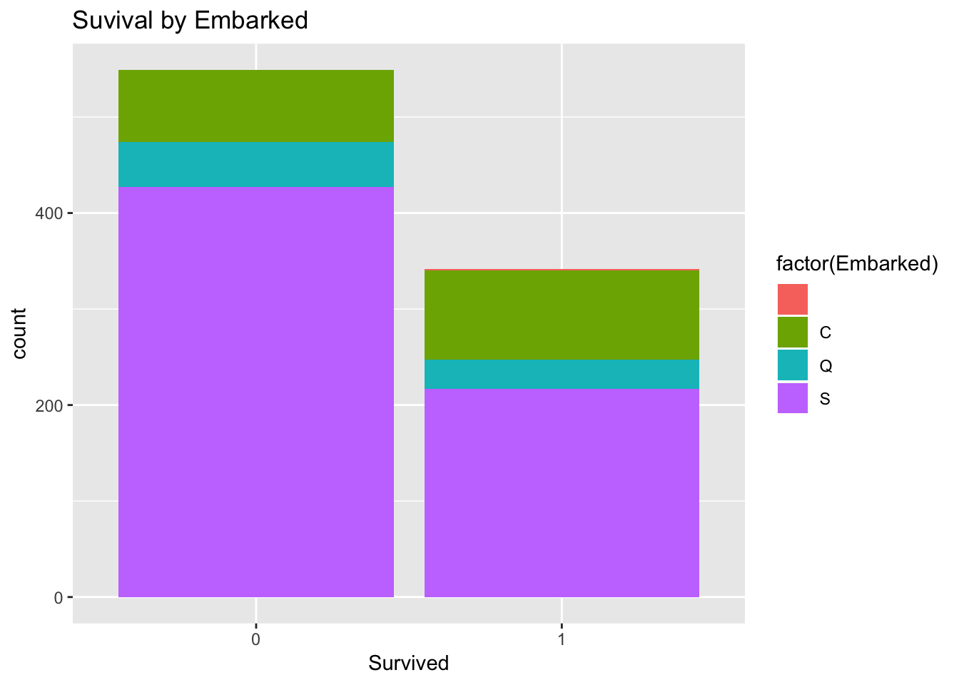
train %>% group_by(Survived, Embarked) %>% summarise(freq = n())
## # A tibble: 7 x 3
## # Groups:   Survived [?]
##   Survived Embarked  freq
##   <fct>    <fct>    <int>
## 1 0        C           75
## 2 0        Q           47
## 3 0        S          427
## 4 1        ""           2
## 5 1        C           93
## 6 1        Q           30
## 7 1        S          217
ggplot(train, aes(x = Survived, fill=factor(Embarked)))+geom_bar()+
  ggtitle("Suvival by Embarked")
Summary 5
차트에 따르면 C에서 탑승한 승객은 살아남을 확률이 높다.
차트에 따르면 Q에서 탑승한 승객은 사망했을 확률이 높다.
차트에 따르면 S에서 탑승한 승객은 사망했을 확률이 높다.
| C | Q | S | |
|---|---|---|---|
| Prob. | 생존>사망 | 생존<사망 | 생존<사망 |
5. Feature engineering
Feature engineering is the process of using domain knowledge of the data
to create features (feature vectors) that make machine learning algorithms work.
feature vector is an n-dimensional vector of numerical features that represent some object.
Many algorithms in machine learning require a numerical representation of objects,
since such representations facilitate processing and statistical analysis.
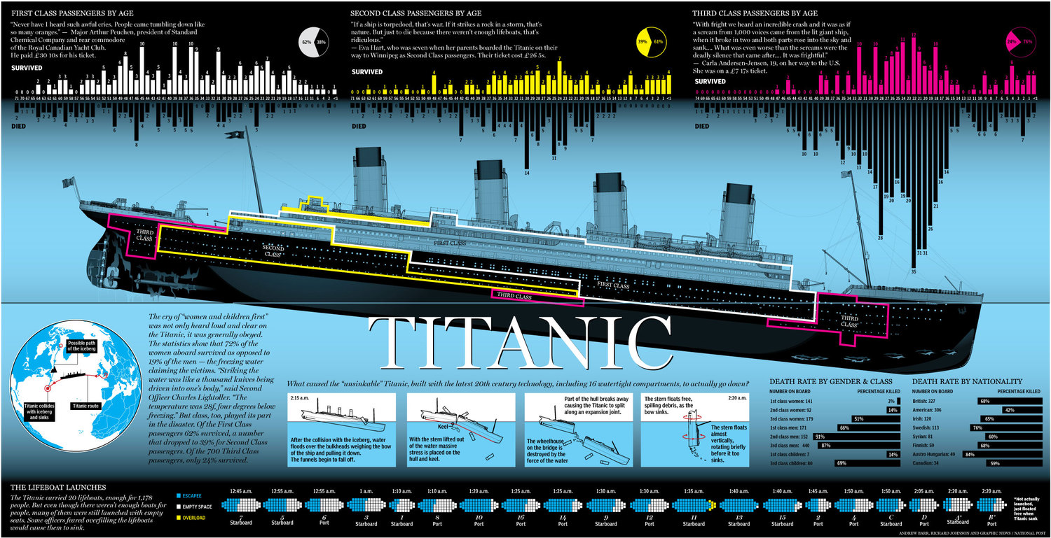
5.1. how titanic sank?
sank from the bow of the ship where third class rooms located
conclusion, Pclass is key feature for classifier
head(train)
##   PassengerId Survived Pclass
## 1           1        0      3
## 2           2        1      1
## 3           3        1      3
## 4           4        1      1
## 5           5        0      3
## 6           6        0      3
##                                                  Name    Sex Age SibSp
## 1                             Braund, Mr. Owen Harris   male  22     1
## 2 Cumings, Mrs. John Bradley (Florence Briggs Thayer) female  38     1
## 3                              Heikkinen, Miss. Laina female  26     0
## 4        Futrelle, Mrs. Jacques Heath (Lily May Peel) female  35     1
## 5                            Allen, Mr. William Henry   male  35     0
## 6                                    Moran, Mr. James   male  NA     0
##   Parch           Ticket    Fare Cabin Embarked
## 1     0        A/5 21171  7.2500              S
## 2     0         PC 17599 71.2833   C85        C
## 3     0 STON/O2. 3101282  7.9250              S
## 4     0           113803 53.1000  C123        S
## 5     0           373450  8.0500              S
## 6     0           330877  8.4583              Q
head(test)
##   PassengerId Pclass                                         Name    Sex
## 1         892      3                             Kelly, Mr. James   male
## 2         893      3             Wilkes, Mrs. James (Ellen Needs) female
## 3         894      2                    Myles, Mr. Thomas Francis   male
## 4         895      3                             Wirz, Mr. Albert   male
## 5         896      3 Hirvonen, Mrs. Alexander (Helga E Lindqvist) female
## 6         897      3                   Svensson, Mr. Johan Cervin   male
##    Age SibSp Parch  Ticket    Fare Cabin Embarked
## 1 34.5     0     0  330911  7.8292              Q
## 2 47.0     1     0  363272  7.0000              S
## 3 62.0     0     0  240276  9.6875              Q
## 4 27.0     0     0  315154  8.6625              S
## 5 22.0     1     1 3101298 12.2875              S
## 6 14.0     0     0    7538  9.2250              S
5.2. Regular expression : Name -> Title
library(stringr)

train['Title'] <- lapply(train['Name'], function(x) str_extract(x, " (([A-Za-z]+))"))
test['Title'] <- lapply(test['Name'], function(x) str_extract(x, " (([A-Za-z]+))"))
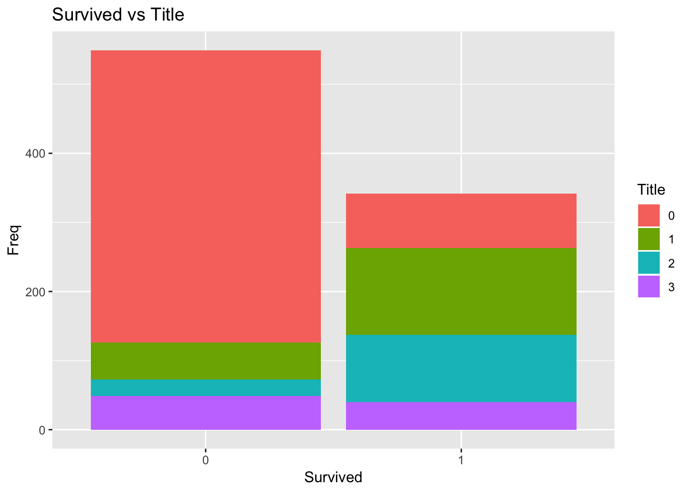
5.3. Convert categorical to numeric variable : Title
feature vector map :
- Mr : 0
- Miss : 1
- Mrs: 2
- Others: 3
train$Title <- ifelse(train$Title == " Mr", 0, ifelse(train$Title == " Miss", 1, ifelse(train$Title == " Mrs", 2, 3)))
test$Title <- ifelse(test$Title == " Mr", 0, ifelse(test$Title == " Miss", 1, ifelse(test$Title == " Mrs", 2, 3)))

train$Title <- as.factor(train$Title)
test$Title <- as.factor(test$Title)


ggplot(train, aes(Survived, fill=Title)) +
  geom_bar() +
  labs(fill = "Title", x = "Survived", y = "Freq",
       title = "Survived vs Title")
#grep("Name", colnames(train))
#grep("Name", colnames(test))

# delete unnecessary feature from dataset
train <- train[, -4]
test <- test[, -3]
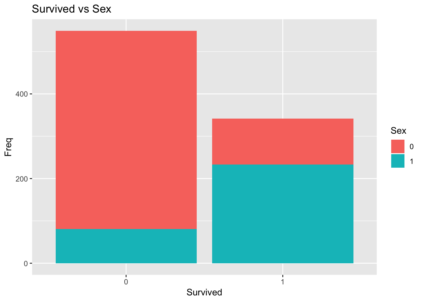
5.4. Convert categorical to numeric variable : Sex
feature vector map :
- male : 0
- female : 1
train$Sex <- ifelse(train$Sex == "male" ,0 , 1)
test$Sex <- ifelse(test$Sex == "male", 0, 1)

train$Sex <- as.factor(train$Sex)
test$Sex <- as.factor(test$Sex)
ggplot(train, aes(Survived, fill=Sex)) +
  geom_bar() +
  labs(fill = "Sex", x = "Survived", y = "Freq",
       title = "Survived vs Sex")
5.5. Convert categorical to numeric variable : Age
5.5.1. some age is missing
Let’s use Title’s median age for missing Age
Trick
- 1. 사람들의 평균 Age
- 2. Title이라는 정보를 활용해서 Title 별 Median Age로 채우기
    - 남자, 결혼한 여성, 미혼 여성
# fill missing age with median age for each title (Mr, Mrs, Miss, Others)
summary(train$Age)
##    Min. 1st Qu.  Median    Mean 3rd Qu.    Max.    NA's
##    0.42   20.12   28.00   29.70   38.00   80.00     177
table(is.na(train$Age))
##
## FALSE  TRUE
##   714   177
summary(test$Age)
##    Min. 1st Qu.  Median    Mean 3rd Qu.    Max.    NA's
##    0.17   21.00   27.00   30.27   39.00   76.00      86
table(is.na(test$Age))
##
## FALSE  TRUE
##   332    86
train %>%
  group_by(Title) %>%                   # class별 분리
  summarise(mean_age = mean(Age, na.rm=TRUE),     # age 평균
            sd_age = sd(Age, na.rm=TRUE),       # age 합계
            median_age = median(Age, na.rm=TRUE), # age 중앙값
            n = n())                    # 탑승객 수
## # A tibble: 4 x 5
##   Title mean_age sd_age median_age     n
##   <fct>    <dbl>  <dbl>      <dbl> <int>
## 1 0         32.4   12.7         30   502
## 2 1         21.8   13.1         21   179
## 3 2         36.2   11.5         35   121
## 4 3         22.5   19.3         18    89
library(doBy)
summaryBy(Age ~ Title, data=test, FUN=c(mean, sd, median), na.rm=TRUE)
##   Title Age.mean   Age.sd Age.median
## 1     0 32.05085 11.98532      28.00
## 2     1 21.64429 10.48901      22.00
## 3     2 39.05000 15.14162      36.50
## 4     3 20.96594 16.35504      13.75
train$Age <- ifelse((is.na(train$Age) & train$Title == 0), 30, train$Age)
train$Age <- ifelse((is.na(train$Age) & train$Title == 1), 21, train$Age)
train$Age <- ifelse((is.na(train$Age) & train$Title == 2), 35, train$Age)
train$Age <- ifelse((is.na(train$Age) & train$Title == 3), 18, train$Age)

test$Age <- ifelse((is.na(test$Age) & test$Title == 0), 28, test$Age)
test$Age <- ifelse((is.na(test$Age) & test$Title == 1), 22, test$Age)
test$Age <- ifelse((is.na(test$Age) & test$Title == 2), 36, test$Age)
test$Age <- ifelse((is.na(test$Age) & test$Title == 3), 13, test$Age)

# 결측치 빈도표 생성
table(is.na(train$Age))
##
## FALSE
##   891
table(is.na(test$Age))
##
## FALSE
##   418
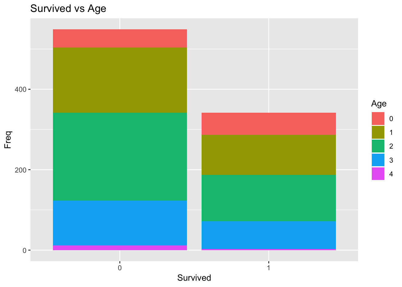
5.5.2. Binning
Binning/Converting Numerical Age to Categorical Variable
feature vector map :
- child : 0  (16세 이하)
- young : 1  (16세 이상 26세 이하)
- adult : 2  (26세 이상 36세 이하)
- mid-age : 3 (36세 이상 62세 이하)
- senior : 4 (62세 이상)
train$Age <- ifelse(train$Age <= 16, 0,
                    ifelse(train$Age > 16 & train$Age <= 26, 1,
                           ifelse(train$Age > 26 & train$Age <= 36, 2,
                                  ifelse(train$Age > 36 & train$Age <= 62, 3, 4))))


test$Age <- ifelse(test$Age <= 16, 0,
                    ifelse(test$Age > 16 & test$Age <= 26, 1,
                           ifelse(test$Age > 26 & test$Age <= 36, 2,
                                  ifelse(test$Age > 36 & test$Age <= 62, 3, 4))))


train$Age <- as.factor(train$Age)
test$Age <- as.factor(test$Age)


ggplot(train, aes(Survived, fill=Age)) +
  geom_bar() +
  labs(fill = "Age", x = "Survived", y = "Freq",
       title = "Survived vs Age")
5.6. Convert categorical to numeric variable : Embarked
5.6.1. filling missing values
table(train$Embarked)
##
##       C   Q   S
##   2 168  77 644
table(train$Pclass)
##
##   1   2   3
## 216 184 491
table(test$Embarked)
##
##   C   Q   S
## 102  46 270
table(test$Pclass)
##
##   1   2   3
## 107  93 218
ggplot(train, aes(Pclass, fill=Embarked)) +
  geom_bar() +
  labs(fill = "Embarked", x = "Pclass", y = "freq",
       title = "Embarked vs Pclass")
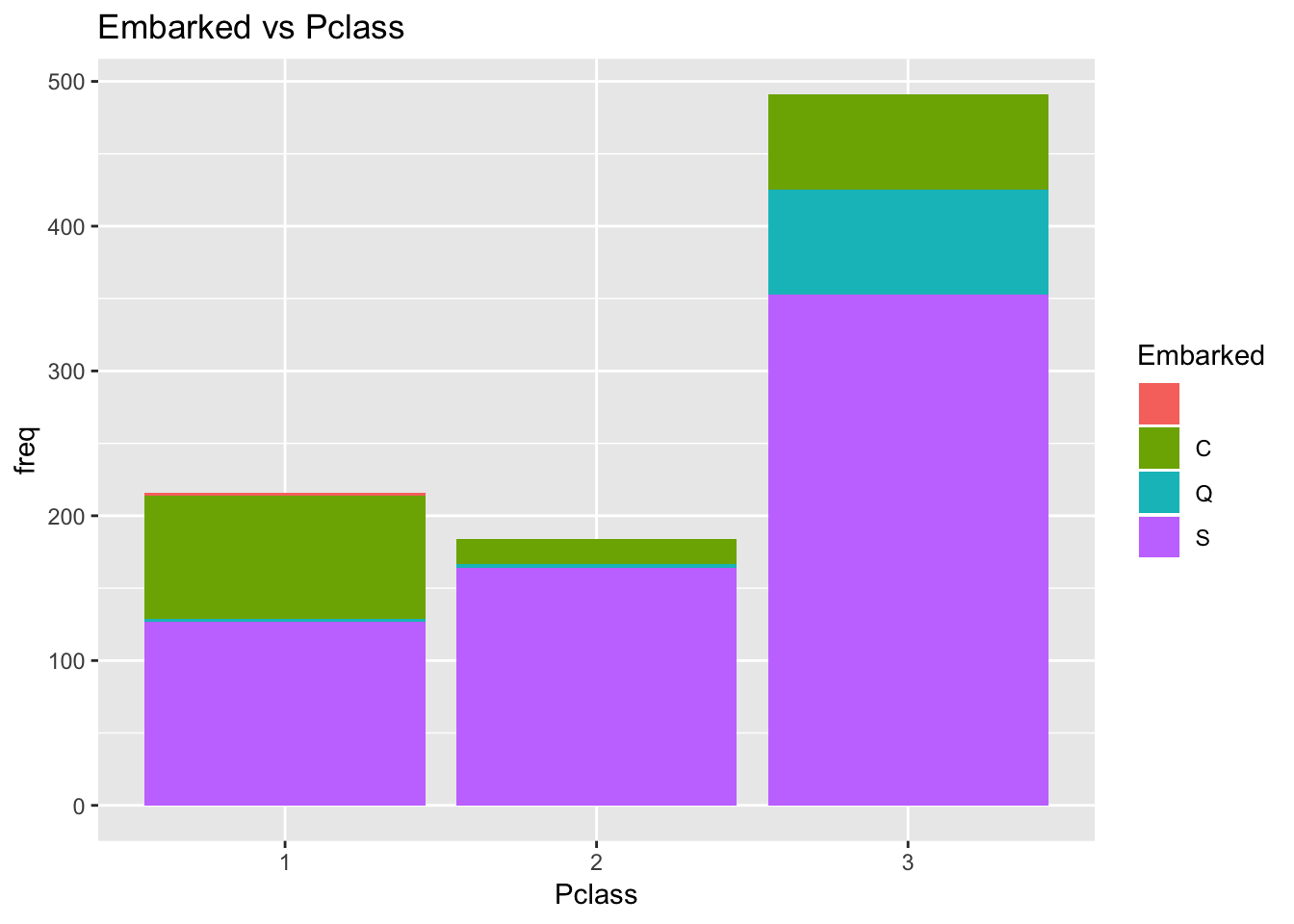
more than 50% of 1st class are from S embark
more than 50% of 2nd class are from S embark
more than 50% of 3rd class are from S embark
fill out missing embark with S embark
5.6.2. Bining
feature vector map :
- C : 0
- Q : 1
- S : 2
# train$Embarked <- ifelse(is.na(train$Embarked), "S", train$Embarked)
train$Embarked <- ifelse(train$Embarked == 0, 4, train$Embarked)
train$Embarked  <- as.factor(as.numeric(train$Embarked) - 1)
test$Embarked <- ifelse(test$Embarked == "C", 0,
                        ifelse(test$Embarked == "Q", 1, 2))

table(train$Embarked)
##
##   0   1   2   3
##   2 168  77 644
table(test$Embarked)
##
##   0   1   2
## 102  46 270
ggplot(train, aes(Pclass, fill=Embarked)) +
  geom_bar() +
  labs(fill = "Embarked", x = "Pclass", y = "freq",
       title = "Embarked vs Pclass")

5.7. Convert categorical to numeric variable : Fare
- 결측치를 처리하는 (통계적인 추론) 방법
- Fare는 Ticket class와 상관관계가 있다.
- 등급별 Fare의 median값으로 missing field를 채워줄 것이다.
5.7.1. filling missing values
# 결측치 빈도표 생성
table(is.na(train$Fare))
##
## FALSE
##   891
table(is.na(test$Fare))
##
## FALSE  TRUE
##   417     1
test %>%
  group_by(Pclass) %>%                   # class별 분리
  summarise(mean_fare = mean(Fare, na.rm=TRUE),     # age 평균
            sd_fare = sd(Fare, na.rm=TRUE),       # age 합계
            median_fare = median(Fare, na.rm=TRUE), # age 중앙값
            n = n())                    # 탑승객 수
## # A tibble: 3 x 5
##   Pclass mean_fare sd_fare median_fare     n
##    <int>     <dbl>   <dbl>       <dbl> <int>
## 1      1      94.3    84.4       60      107
## 2      2      22.2    14.0       15.8     93
## 3      3      12.5    10.8        7.90   218
test$Fare <- ifelse((is.na(test$Fare) & test$Pclass == 1), 60, test$Fare)
test$Fare <- ifelse((is.na(test$Fare) & test$Pclass == 2), 15.75, test$Fare)
test$Fare <- ifelse((is.na(test$Fare) & test$Pclass == 3), 7.89, test$Fare)

# 결측치 빈도표 생성
table(is.na(train$Fare))
##
## FALSE
##   891
table(is.na(test$Fare))
##
## FALSE
##   418
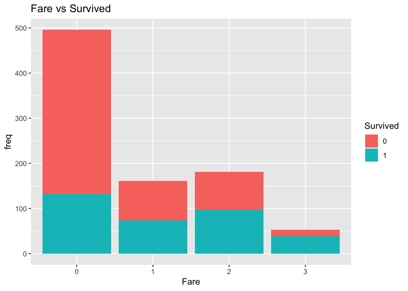
5.7.2. Binning
Binning/Converting Numerical Fare to Categorical Variable
feature vector map:
- 17달러 이하 : 0
- 17~30달러 : 1
- 30~100 달러 : 2
- 100달러 이상 : 3
train$Fare <- ifelse(train$Fare <= 17, 0,
                    ifelse(train$Fare > 17 & train$Fare <= 30, 1,
                           ifelse(train$Fare > 30 & train$Fare <= 100, 2, 3)))


test$Fare <- ifelse(test$Fare <= 17, 0,
                    ifelse(test$Fare > 17 & test$Fare <= 30, 1,
                           ifelse(test$Fare > 30 & test$Fare <= 100, 2, 3)))


train$Fare <- as.factor(train$Fare)
test$Fare <- as.factor(test$Fare)

table(train$Fare)
##
##   0   1   2   3
## 496 161 181  53
table(test$Fare)
##
##   0   1   2   3
## 236  73  78  31
ggplot(train, aes(Fare, fill=Survived)) +
  geom_bar() +
  labs(fill = "Survived", x = "Fare", y = "freq",
       title = "Fare vs Survived")


5.8. Convert categorical to numeric variable : Cabin
- 호텔의 방 같은 개념
train['Cabin'] <- lapply(train['Cabin'], function(x) str_extract(x, substr(x, 1, 1)))
test['Cabin']  <- lapply(test['Cabin'], function(x) str_extract(x, substr(x, 1, 1)))

ggplot(train, aes(Pclass, fill=Cabin)) +
  geom_bar() +
  labs(fill = "Cabin", x = "Pclass", y = "freq",
       title = "Pclass vs Cabin")
Feature scailing
- 소수점을 사용하는 이유는 기본적으로 ML 분류기는 숫자를 사용하고, 계산할 때 보통 유클리디안 거리를 쓴다.
- 숫자의 범위가 비슷하지 않으면, 큰 거리에 있는 것을 조금 더 중요하게 생각할 수 있다.
- 예를 들면, 성별은 0, 1 밖에 없는데 티켓의 가격은 10달러, 20달러 티켓이 있다고 가정해보자.
- 10 달러, 20달러 티켓은 3등급이라고 생각해보면, 별로 다를 게 없다. 하지만 남자와 여자는 완전히 다르지만 1-0 이라 1 차이이고, 10달러 20달러는 차이는 10이다. 우리가 같은 range를 주지 않았을 경우 바보같은 Machine Learning Classifier는 10달러 차이가 남자하고 여자 차이보다 더 크게 느껴질 것이다. 해서 범위를 비슷하게 주기 위해서 소수점을 사용했다. 이 테크닉을 feature Scailng이라고 한다.
train$Cabin <- ifelse(train$Cabin == "A", 0,
                      ifelse(train$Cabin == "B", 0.4,
                             ifelse(train$Cabin == "C", 0.8,
                                    ifelse(train$Cabin == "D", 1.2,
                                           ifelse(train$Cabin == "E", 1.6,
                                                  ifelse(train$Cabin == "F", 2,
                                                         ifelse(train$Cabin == "G", 2.4,2.8)))))))

test$Cabin <- ifelse(test$Cabin == "A", 0,
                      ifelse(test$Cabin == "B", 0.4,
                             ifelse(test$Cabin == "C", 0.8,
                                    ifelse(test$Cabin == "D", 1.2,
                                           ifelse(test$Cabin == "E", 1.6,
                                                  ifelse(test$Cabin == "F", 2,
                                                         ifelse(test$Cabin == "G", 2.4,2.8)))))))

# train$Cabin <- as.factor(train$Cabin)
# test$Cabin <- as.factor(test$Cabin)
방의 위치는 Class와 밀접한 연관이 있기 때문에 각 클래스별 Cabin의 중간값을 missing value에 넣어준다.
summary(train$Cabin)
##    Min. 1st Qu.  Median    Mean 3rd Qu.    Max.    NA's
##  0.0000  0.4000  0.8000  0.9569  1.2000  2.8000     687
# 결측치 빈도표 생성
table(is.na(train$Cabin))
##
## FALSE  TRUE
##   204   687
table(is.na(test$Cabin))
##
## FALSE  TRUE
##    91   327
train %>%
  group_by(Pclass) %>%                   # class별 분리
  summarise(mean_Cabin = mean(Cabin, na.rm=TRUE),     # age 평균
            sd_Cabin = sd(Cabin, na.rm=TRUE),       # age 합계
            median_Cabin = median(Cabin, na.rm=TRUE), # age 중앙값
            n = n())                    # 탑승객 수
## # A tibble: 3 x 5
##   Pclass mean_Cabin sd_Cabin median_Cabin     n
##   <fct>       <dbl>    <dbl>        <dbl> <int>
## 1 1           0.816    0.488          0.8   216
## 2 2           1.7      0.343          1.8   184
## 3 3           2.03     0.317          2     491
test %>%
  group_by(Pclass) %>%                   # class별 분리
  summarise(mean_Cabin = mean(Cabin, na.rm=TRUE),     # age 평균
            sd_Cabin = sd(Cabin, na.rm=TRUE),       # age 합계
            median_Cabin = median(Cabin, na.rm=TRUE), # age 중앙값
            n = n())                    # 탑승객 수
## # A tibble: 3 x 5
##   Pclass mean_Cabin sd_Cabin median_Cabin     n
##    <int>      <dbl>    <dbl>        <dbl> <int>
## 1      1      0.785    0.434          0.8   107
## 2      2      1.77     0.390          2      93
## 3      3      2.1      0.200          2     218
# fill missing Fare with median fare for each Pclass
train$Cabin <- ifelse((is.na(train$Cabin) & train$Pclass == 1), 0.8, train$Cabin)
train$Cabin <- ifelse((is.na(train$Cabin) & train$Pclass == 2), 1.8, train$Cabin)
train$Cabin <- ifelse((is.na(train$Cabin) & train$Pclass == 3), 2.0, train$Cabin)

test$Cabin <- ifelse((is.na(test$Cabin) & test$Pclass == 1), 0.8, test$Cabin)
test$Cabin <- ifelse((is.na(test$Cabin) & test$Pclass == 2), 2.0, test$Cabin)
test$Cabin <- ifelse((is.na(test$Cabin) & test$Pclass == 3), 2.0, test$Cabin)


# 결측치 빈도표 생성
table(is.na(train$Cabin))
##
## FALSE
##   891
table(is.na(test$Cabin))
##
## FALSE
##   418
5.9. FamilySize
train['FamilySize'] <- train["SibSp"] + train["Parch"] + 1
test['FamilySize'] <- test["SibSp"] + test["Parch"] + 1

table(train['FamilySize'])
##
##   1   2   3   4   5   6   7   8  11
## 537 161 102  29  15  22  12   6   7
table(test['FamilySize'])
##
##   1   2   3   4   5   6   7   8  11
## 253  74  57  14   7   3   4   2   4
library(DescTools)
Desc(train['FamilySize'])
## -------------------------------------------------------------------------
## Describe train["FamilySize"] (data.frame):
##
## data.frame:  891 obs. of  1 variables
##
##   Nr  ColName     Class    NAs  Levels
##   1   FamilySize  numeric  .
##
##
## -------------------------------------------------------------------------
## 1 - FamilySize (numeric)
##
##   length       n    NAs  unique    0s  mean  meanCI
##      891     891      0       9     0  1.90    1.80
##           100.0%   0.0%          0.0%          2.01
##
##      .05     .10    .25  median   .75   .90     .95
##     1.00    1.00   1.00    1.00  2.00  4.00    6.00
##
##    range      sd  vcoef     mad   IQR  skew    kurt
##    10.00    1.61   0.85    0.00  1.00  2.72    9.07
##
##
##    level  freq   perc  cumfreq  cumperc
## 1      1   537  60.3%      537    60.3%
## 2      2   161  18.1%      698    78.3%
## 3      3   102  11.4%      800    89.8%
## 4      4    29   3.3%      829    93.0%
## 5      5    15   1.7%      844    94.7%
## 6      6    22   2.5%      866    97.2%
## 7      7    12   1.3%      878    98.5%
## 8      8     6   0.7%      884    99.2%
## 9     11     7   0.8%      891   100.0%
Desc(test['FamilySize'])
## -------------------------------------------------------------------------
## Describe test["FamilySize"] (data.frame):
##
## data.frame:  418 obs. of  1 variables
##
##   Nr  ColName     Class    NAs  Levels
##   1   FamilySize  numeric  .
##
##
## -------------------------------------------------------------------------
## 1 - FamilySize (numeric)
##
##   length       n    NAs  unique    0s  mean  meanCI
##      418     418      0       9     0  1.84    1.69
##           100.0%   0.0%          0.0%          1.99
##
##      .05     .10    .25  median   .75   .90     .95
##     1.00    1.00   1.00    1.00  2.00  3.00    4.00
##
##    range      sd  vcoef     mad   IQR  skew    kurt
##    10.00    1.52   0.83    0.00  1.00  3.15   13.18
##
##
##    level  freq   perc  cumfreq  cumperc
## 1      1   253  60.5%      253    60.5%
## 2      2    74  17.7%      327    78.2%
## 3      3    57  13.6%      384    91.9%
## 4      4    14   3.3%      398    95.2%
## 5      5     7   1.7%      405    96.9%
## 6      6     3   0.7%      408    97.6%
## 7      7     4   1.0%      412    98.6%
## 8      8     2   0.5%      414    99.0%
## 9     11     4   1.0%      418   100.0%
head(train)
##   PassengerId Survived Pclass Sex Age SibSp Parch           Ticket Fare
## 1           1        0      3   0   1     1     0        A/5 21171    0
## 2           2        1      1   1   3     1     0         PC 17599    2
## 3           3        1      3   1   1     0     0 STON/O2. 3101282    0
## 4           4        1      1   1   2     1     0           113803    2
## 5           5        0      3   0   2     0     0           373450    0
## 6           6        0      3   0   2     0     0           330877    0
##   Cabin Embarked Title FamilySize
## 1   2.0        3     0          2
## 2   0.8        1     2          2
## 3   2.0        3     1          1
## 4   0.8        3     2          2
## 5   2.0        3     0          1
## 6   2.0        2     0          1
head(test)
##   PassengerId Pclass Sex Age SibSp Parch  Ticket Fare Cabin Embarked Title
## 1         892      3   0   2     0     0  330911    0     2        1     0
## 2         893      3   1   3     1     0  363272    0     2        2     2
## 3         894      2   0   3     0     0  240276    0     2        1     0
## 4         895      3   0   2     0     0  315154    0     2        2     0
## 5         896      3   1   1     1     1 3101298    0     2        2     2
## 6         897      3   0   0     0     0    7538    0     2        2     0
##   FamilySize
## 1          1
## 2          2
## 3          1
## 4          1
## 5          3
## 6          1
6. Modeling 1 : Decision Tree- C5.0 Algorithm
6.1. data preparation - creating random training and test datasets
- 데이터의 수에 따라 Train / Test의 비율을 6:4~9:1로 정한다.
- 훈련 데이터셋과 테스트 데이터셋을 9:1로 정했고, 각 데이터셋은 약 30%의 채무 불이행 대출을 가졌다.
train <- train[, -c(1, 6, 7, 8)]
test <- test[, -c(1, 5, 6, 7)]
target <- train[, 1]

head(train)
##   Survived Pclass Sex Age Fare Cabin Embarked Title FamilySize
## 1        0      3   0   1    0   2.0        3     0          2
## 2        1      1   1   3    2   0.8        1     2          2
## 3        1      3   1   1    0   2.0        3     1          1
## 4        1      1   1   2    2   0.8        3     2          2
## 5        0      3   0   2    0   2.0        3     0          1
## 6        0      3   0   2    0   2.0        2     0          1
head(test)
##   Pclass Sex Age Fare Cabin Embarked Title FamilySize
## 1      3   0   2    0     2        1     0          1
## 2      3   1   3    0     2        2     2          2
## 3      2   0   3    0     2        1     0          1
## 4      3   0   2    0     2        2     0          1
## 5      3   1   1    0     2        2     2          3
## 6      3   0   0    0     2        2     0          1
# create a random sample for training and test data
# use set.seed to use the same random number sequence as the tutorial
set.seed(1606)

n <- nrow(train)
idx <- 1:n

training_idx <- sample(idx, n * .80)
idx <- setdiff(idx, training_idx)
validate_idx <- sample(idx, n * .20)
# test_idx <- setdiff(idx, validate_idx)

# split the data frames
train_data <- train[training_idx,]
valid_data <- train[validate_idx,]

target_train <- train_data[, 1]
target_valid <- valid_data[, 1]

train_data <- train_data[, -1]
valid_data <- valid_data[, -1]
test_data <- test
# check the proportion of class variable
table(target_train)
## target_train
##   0   1
## 434 278
prop.table(table(target_train))
## target_train
##         0         1
## 0.6095506 0.3904494
table(target_valid)
## target_valid
##   0   1
## 115  63
prop.table(table(target_valid))
## target_valid
##         0         1
## 0.6460674 0.3539326
dim(train_data)
## [1] 712 8
dim(valid_data)
## [1] 178 8
dim(test_data)
## [1] 418 8
6.2. training a model on the data - C5.0 Decision Trees
# build the simplest decision tree
data_model <- C5.0(train_data, target_train)

# display simple facts about the tree
data_model
##
## Call:
## C5.0.default(x = train_data, y = target_train)
##
## Classification Tree
## Number of samples: 712
## Number of predictors: 8
##
## Tree size: 13
##
## Non-standard options: attempt to group attributes
# display detailed information about the tree
summary(data_model)
##
## Call:
## C5.0.default(x = train_data, y = target_train)
##
##
## C5.0 [Release 2.07 GPL Edition]      Thu Oct 11 07:14:42 2018
## -------------------------------
##
## Class specified by attribute `outcome'
##
## Read 712 cases (9 attributes) from undefined.data
##
## Decision tree:
##
## Sex = 0:
## :...Title in {0,1,2}: 0 (403/66)
## :   Title = 3:
## :   :...FamilySize > 5: 0 (11/1)
## :       FamilySize <= 5:
## :       :...FamilySize <= 2: 0 (28/8)
## :           FamilySize > 2: 1 (21/3)
## Sex = 1:
## :...Pclass in {1,2}: 1 (136/5)
##     Pclass = 3:
##     :...FamilySize > 4: 0 (21/2)
##         FamilySize <= 4:
##         :...Age = 3: 0 (6)
##             Age in {0,1,2,4}:
##             :...Embarked in {0,2}: 1 (28/8)
##                 Embarked = 3:
##                 :...Title in {1,3}: 0 (31/13)
##                 :   Title in {0,2}: 1 (12/3)
##                 Embarked = 1:
##                 :...Fare in {1,2,3}: 1 (6)
##                     Fare = 0:
##                     :...FamilySize <= 1: 1 (3)
##                         FamilySize > 1: 0 (6/1)
##
##
## Evaluation on training data (712 cases):
##
##      Decision Tree
##    ----------------
##    Size      Errors
##
##      13  110(15.4%)   <<
##
##
##     (a)   (b)    <-classified as
##    ----  ----
##     415    19    (a): class 0
##      91   187    (b): class 1
##
##
##  Attribute usage:
##
##  100.00% Sex
##   71.07% Title
##   34.97% Pclass
##   24.30% FamilySize
##   12.92% Age
##   12.08% Embarked
##    2.11% Fare
##
##
## Time: 0.0 secs
6.3. Summary : Decision Tree (C5.0)
Evaluation on training data (712 cases):

        Decision Tree
      ----------------
      Size      Errors

        13  110(15.4%)   <<


       (a)   (b)    <-classified as
      ----  ----
       415    19    (a): class 0
        91   187    (b): class 1


    Attribute usage:

    100.00% Sex
     71.07% Title
     34.97% Pclass
     24.30% FamilySize
     12.92% Age
     12.08% Embarked
      2.11% Fare
Errors 출력은 모델이 15.4%의 오류율로 712개의 훈련 인스턴스 중 110개를 제외하고 전부 정확하게 분류했음을 말하고 있다.
총 19개의 실제 0(Dead)값은 1(Survived)로 부정확하게 분류된 반면(거짓 긍정), 91개의 1(Survived) 값은 0(Dead)로 오분류 됐다(거짓 부정).
의사결정 트리는 모델을 훈련 데이터에 과적합 시키는 경향이 있는 것으로 알려져 있다. 이런 이유로 훈련 데이터에 대해 보고된 오류율은 매우 낙관적일 수 있으며, 테스트 데이터셋에 대해 의사결정 트리를 평가하는 것은 중요하다.
train_pred <- predict(data_model, train_data)
confusionMatrix(target_train, train_pred)
## Confusion Matrix and Statistics
##
##           Reference
## Prediction   0   1
##          0 415  19
##          1  91 187
##
##                Accuracy : 0.8455
##                  95% CI : (0.8168, 0.8713)
##     No Information Rate : 0.7107
##     P-Value [Acc > NIR] : < 2.2e-16
##
##                   Kappa : 0.6596
##  Mcnemar's Test P-Value : 1.292e-11
##
##             Sensitivity : 0.8202
##             Specificity : 0.9078
##          Pos Pred Value : 0.9562
##          Neg Pred Value : 0.6727
##              Prevalence : 0.7107
##          Detection Rate : 0.5829
##    Detection Prevalence : 0.6096
##       Balanced Accuracy : 0.8640
##
##        'Positive' Class : 0
##
6.4. Evaluating model performance
## Evaluating model performance
# create a factor vector of predictions on test data
data_pred <- predict(data_model, valid_data)
# cross tabulation of predicted versus actual classes
CrossTable(target_valid, data_pred,
           prop.chisq = FALSE, prop.c = FALSE, prop.r = FALSE,
           dnn = c('actual survived', 'predicted survived'))
##
##
##    Cell Contents
## |-------------------------|
## |                       N |
## |         N / Table Total |
## |-------------------------|
##
##
## Total Observations in Table:  178
##
##
##                 | predicted survived
## actual survived |         0 |         1 | Row Total |
## ----------------|-----------|-----------|-----------|
##               0 |       104 |        11 |       115 |
##                 |     0.584 |     0.062 |           |
## ----------------|-----------|-----------|-----------|
##               1 |        24 |        39 |        63 |
##                 |     0.135 |     0.219 |           |
## ----------------|-----------|-----------|-----------|
##    Column Total |       128 |        50 |       178 |
## ----------------|-----------|-----------|-----------|
##
##
confusionMatrix(target_valid, data_pred)
## Confusion Matrix and Statistics
##
##           Reference
## Prediction   0   1
##          0 104  11
##          1  24  39
##
##                Accuracy : 0.8034
##                  95% CI : (0.7373, 0.8591)
##     No Information Rate : 0.7191
##     P-Value [Acc > NIR] : 0.006396
##
##                   Kappa : 0.549
##  Mcnemar's Test P-Value : 0.042522
##
##             Sensitivity : 0.8125
##             Specificity : 0.7800
##          Pos Pred Value : 0.9043
##          Neg Pred Value : 0.6190
##              Prevalence : 0.7191
##          Detection Rate : 0.5843
##    Detection Prevalence : 0.6461
##       Balanced Accuracy : 0.7963
##
##        'Positive' Class : 0
##
6.5. Summary : Test 평가 지표
178개 테스트 레코드 중에서 실제 104명은 사망하였고, 39명은 생존했음을 모델이 정확하게 예측해서 정확도는 80.3%이고, 오류율은 19.7%가 됐다.
처음 보는 데이터에 대해 모델 성능이 더 나빠진다는 점을 감안하면 이 결과가 훈련 데이터에 대한 성능보다 다소 나쁘기는 하지만 전혀 예상 밖인 것은 아니다. 또한 모델이 테스트 데이터에서 실제 115명의 사망자 중 104명(90.4%)를 정확하게 예측했지만, 나머지 11명(9.5%)는 생존한다고 예측했으나 죽었다는 점을 주목하자.
유감스럽게도 이런 오류 유형은 잠재적으로 비용이 매우 많이 드는 실수다. 더 노력해서 결과를 개선할 수 있는지 살펴보겠다.
6.6. Improving model performance
모델 성능 개선의 필요성
6.6.1. Boosting the accuracy of decision trees (의사결정 트리의 정확도 향상)
C5.0 알고리즘이 C4.5 알고리즘을 개선한 방법 중 하나는 적응형 부스팅(AdaBoost)을 추가한 것이다. 이 방법은 여러 개의 의사결정 트리를 만들어서 각 예시에 대해 최고 클래스를 투표하게 만드는 과정이다.
부스팅은 성능이 약한 여러 학습자를 결헙함으로써 어느 한 학습자 혼자보다 훨씬 강한 팀을 만들 수 있다는 생각에 뿌리를 두고 있다. 각 모델은 각자의 유일한 강점과 약점을 찾으며, 특정 문제를 풀 때 더 좋거나 더 나쁠 수 있다. 그러므로 상호 보완적인 장점과 단점을 갖는 여러 학습자를 조합해 분류기의 정확도를 극적으로 향상시킬 수 있다.
부스팅 팀에 사용할 독립적인 의사결정 트리의 개수를 나타내는 trials 파라미터를 간단히 추가한다. trials 파라미터는 상한선을 설정한다. 추가 시행이 정확도를 향상시키지 못할 것으로 보이면 알고리즘은 더 이상 트리를 추가하지 않는다.
10회 시행으로 시작할 것인데, 연구에 따르면 10회 시행 시 테스트 데이터에 대한 오류율이 약 25% 정도 줄기때문에 이 숫자는 사실상 표준이 된 상태다.
## Improving model performance
## Boosting the accuracy of decision trees
# boosted decision tree with 10 trials
data_boost10 <- C5.0(train_data, target_train,
                       trials = 10)
data_boost10
##
## Call:
## C5.0.default(x = train_data, y = target_train, trials = 10)
##
## Classification Tree
## Number of samples: 712
## Number of predictors: 8
##
## Number of boosting iterations: 10
## Average tree size: 7.6
##
## Non-standard options: attempt to group attributes
summary(data_boost10)
##
## Call:
## C5.0.default(x = train_data, y = target_train, trials = 10)
##
##
## C5.0 [Release 2.07 GPL Edition]      Thu Oct 11 07:14:42 2018
## -------------------------------
##
## Class specified by attribute `outcome'
##
## Read 712 cases (9 attributes) from undefined.data
##
## -----  Trial 0:  -----
##
## Decision tree:
##
## Sex = 0:
## :...Title in {0,1,2}: 0 (403/66)
## :   Title = 3:
## :   :...FamilySize > 5: 0 (11/1)
## :       FamilySize <= 5:
## :       :...FamilySize <= 2: 0 (28/8)
## :           FamilySize > 2: 1 (21/3)
## Sex = 1:
## :...Pclass in {1,2}: 1 (136/5)
##     Pclass = 3:
##     :...FamilySize > 4: 0 (21/2)
##         FamilySize <= 4:
##         :...Age = 3: 0 (6)
##             Age in {0,1,2,4}:
##             :...Embarked in {0,2}: 1 (28/8)
##                 Embarked = 3:
##                 :...Title in {1,3}: 0 (31/13)
##                 :   Title in {0,2}: 1 (12/3)
##                 Embarked = 1:
##                 :...Fare in {1,2,3}: 1 (6)
##                     Fare = 0:
##                     :...FamilySize <= 1: 1 (3)
##                         FamilySize > 1: 0 (6/1)
##
## -----  Trial 1:  -----
##
## Decision tree:
##
## Cabin <= 1.6: 1 (206.2/56.5)
## Cabin > 1.6:
## :...Sex = 0: 0 (337.8/89.5)
##     Sex = 1:
##     :...Pclass in {1,2}: 1 (43.2/4.2)
##         Pclass = 3:
##         :...FamilySize <= 4: 1 (105.5/46.4)
##             FamilySize > 4: 0 (19.4/4.2)
##
## -----  Trial 2:  -----
##
## Decision tree:
##
## Title = 0: 0 (407.5/145.1)
## Title in {1,2,3}:
## :...Pclass in {1,2}: 1 (135.3/25.5)
##     Pclass = 3: 0 (169.2/74.5)
##
## -----  Trial 3:  -----
##
## Decision tree:
##
## Sex = 1:
## :...Pclass in {1,2}: 1 (92.8/14.8)
## :   Pclass = 3:
## :   :...Title in {0,1}: 1 (103.6/46.4)
## :       Title in {2,3}: 0 (41.5/18.7)
## Sex = 0:
## :...Embarked = 1: 1 (96.7/43.6)
##     Embarked in {0,2}: 0 (28.4/8.9)
##     Embarked = 3:
##     :...Age in {1,3,4}: 0 (161.6/54.3)
##         Age = 0: 1 (36/11.1)
##         Age = 2:
##         :...Fare = 0: 0 (90.2/34)
##             Fare in {1,2,3}: 1 (61.2/25.5)
##
## -----  Trial 4:  -----
##
## Decision tree:
##
## Sex = 1: 1 (236.1/93.1)
## Sex = 0:
## :...Pclass in {2,3}: 0 (326.2/135.2)
##     Pclass = 1:
##     :...Cabin > 0.8: 1 (38.4/12.8)
##         Cabin <= 0.8:
##         :...FamilySize <= 2: 0 (99.7/38.9)
##             FamilySize > 2: 1 (11.6/3.4)
##
## -----  Trial 5:  -----
##
## Decision tree:
##
## FamilySize > 4: 0 (44/10.7)
## FamilySize <= 4:
## :...Age = 0: 1 (62.9/14.8)
##     Age in {1,2,3,4}:
##     :...Fare in {2,3}: 1 (152.8/59.5)
##         Fare in {0,1}:
##         :...Age in {3,4}: 0 (93.5/32.8)
##             Age = 1:
##             :...Embarked = 1: 1 (22.1/4.7)
##             :   Embarked in {0,2,3}: 0 (137.3/60.6)
##             Age = 2:
##             :...Embarked in {0,1}: 0 (33.6/8.6)
##                 Embarked in {2,3}:
##                 :...Fare = 1: 1 (40.3/15.9)
##                     Fare = 0:
##                     :...Pclass = 1: 0 (2.8)
##                         Pclass in {2,3}:
##                         :...Cabin <= 1.6: 1 (8)
##                             Cabin > 1.6: 0 (114.7/49.7)
##
## -----  Trial 6:  -----
##
## Decision tree:
##
## Title = 0: 0 (370.6/134.8)
## Title in {1,2,3}:
## :...Pclass in {1,2}: 1 (121.5/28.7)
##     Pclass = 3:
##     :...FamilySize <= 4: 1 (172.3/78.9)
##         FamilySize > 4: 0 (33.6/9.8)
##
## -----  Trial 7:  -----
##
## Decision tree:
##
## Cabin > 1.6:
## :...Title = 0: 0 (168.4/28.4)
## :   Title in {1,2,3}:
## :   :...Pclass = 2: 1 (55.7/15)
## :       Pclass in {1,3}: 0 (225.7/83.9)
## Cabin <= 1.6:
## :...Sex = 1: 1 (38.6)
##     Sex = 0:
##     :...Age = 4: 0 (6)
##         Age in {0,1,2,3}:
##         :...Cabin <= 0.8: 0 (122.1/55.8)
##             Cabin > 0.8: 1 (60.5/18.3)
##
## -----  Trial 8:  -----
##
## Decision tree:
##
## Sex = 0:
## :...Cabin > 1.6: 0 (191.5/27.5)
## :   Cabin <= 1.6:
## :   :...Age in {0,2}: 1 (90.3/31.4)
## :       Age in {1,4}: 0 (29.1/11.3)
## :       Age = 3:
## :       :...Cabin <= 0: 1 (9.6/1.4)
## :           Cabin > 0: 0 (69/27.8)
## Sex = 1:
## :...Pclass in {1,2}: 1 (60.2)
##     Pclass = 3:
##     :...FamilySize > 4: 0 (14.2)
##         FamilySize <= 4:
##         :...Age in {0,1,2,4}: 1 (191.4/79.6)
##             Age = 3: 0 (10.7)
##
## -----  Trial 9:  -----
##
## Decision tree:
##
## Title = 0:
## :...Cabin > 1.6: 0 (105.4)
## :   Cabin <= 1.6:
## :   :...FamilySize <= 2: 0 (159/59.7)
## :       FamilySize > 2: 1 (24.3/7.5)
## Title in {1,2,3}:
## :...FamilySize > 4: 0 (19.7/3.1)
##     FamilySize <= 4:
##     :...Age in {0,4}: 1 (74.1/7.5)
##         Age in {1,2,3}:
##         :...Embarked in {0,1,2}: 1 (89.2/21.5)
##             Embarked = 3:
##             :...Cabin <= 1.6: 1 (25.8/5)
##                 Cabin > 1.6:
##                 :...Sex = 0: 0 (22.6)
##                     Sex = 1:
##                     :...Pclass = 2: 1 (18.1)
##                         Pclass in {1,3}: 0 (108.8/36.1)
##
##
## Evaluation on training data (712 cases):
##
## Trial        Decision Tree
## -----      ----------------
##    Size      Errors
##
##    0     13  110(15.4%)
##    1      5  161(22.6%)
##    2      3  150(21.1%)
##    3      9  196(27.5%)
##    4      5  153(21.5%)
##    5     11  190(26.7%)
##    6      4  137(19.2%)
##    7      7  149(20.9%)
##    8      9  135(19.0%)
##    9     10  124(17.4%)
## boost            102(14.3%)   <<
##
##
##     (a)   (b)    <-classified as
##    ----  ----
##     404    30    (a): class 0
##      72   206    (b): class 1
##
##
##  Attribute usage:
##
##  100.00% Pclass
##  100.00% Sex
##  100.00% Cabin
##  100.00% Title
##  100.00% FamilySize
##   96.07% Age
##   94.66% Embarked
##   87.22% Fare
##
##
## Time: 0.0 secs
10회의 반복을 통해 트리의 크기가 줄어들었다.

Evaluation on training data (712 cases):

Trial       Decision Tree
-----     ----------------
      Size      Errors

   0        13  110(15.4%)
   1         5  161(22.6%)
   2         3  150(21.1%)
   3         9  196(27.5%)
   4         5  153(21.5%)
   5        11  190(26.7%)
   6         4  137(19.2%)
   7         7  149(20.9%)
   8         9  135(19.0%)
   9        10  124(17.4%)
boost           102(14.3%)   <<


       (a)   (b)    <-classified as
      ----  ----
       404    30    (a): class 0
        72   206    (b): class 1


    Attribute usage:

    100.00% Pclass
    100.00% Sex
    100.00% Cabin
    100.00% Title
    100.00% FamilySize
     96.07% Age
     94.66% Embarked
     87.22% Fare
data_boost_pred10 <- predict(data_boost10, valid_data)
CrossTable(target_valid, data_boost_pred10,
           prop.chisq = FALSE, prop.c = FALSE, prop.r = FALSE,
           dnn = c('actual default', 'predicted default'))
##
##
##    Cell Contents
## |-------------------------|
## |                       N |
## |         N / Table Total |
## |-------------------------|
##
##
## Total Observations in Table:  178
##
##
##                | predicted default
## actual default |         0 |         1 | Row Total |
## ---------------|-----------|-----------|-----------|
##              0 |       103 |        12 |       115 |
##                |     0.579 |     0.067 |           |
## ---------------|-----------|-----------|-----------|
##              1 |        18 |        45 |        63 |
##                |     0.101 |     0.253 |           |
## ---------------|-----------|-----------|-----------|
##   Column Total |       121 |        57 |       178 |
## ---------------|-----------|-----------|-----------|
##
##
6.6.2. Summary : Boosting model
- 이 결과를 보면 전체 오류율이 부스팅 이전 19.7%에서 부스팅 모델의 16.8%로 줄어들었다.
- 이득이 큰 것처럼 보이지 않을 수도 있겠지만, 15% 정도 감소한 것이다.
- 한편으로 모델은 사망을 45/57 = 78.9% 정도 정확히 예측하고 있다.
- 12/57 = 21%를 줄이면 더 좋지만 개선이 쉽지 않다.
- 더 크게 개선되지 않는 이유는 상대적으로 작은 훈련 데이터셋과 함수 관계에 있거나, 이 문제가 원래 해결하기 매우 어려운 문제이기 때문일 수도 있다.
- “부스팅이 이렇게 쉽게 추가될 수 있다면 왜 모든 의사결정 트리에 디폴트로 적용하지 않는가?”
- 두 가지 이유가 있다.
- 첫째, 의사결정 트리를 한 번 만드는데 계산 시간이 많이 걸린다면 여러 개의 트리를 만드는 것은 계산적으로 비현실적일 수 있다.
- 둘째, 훈련 데이터에 잡음이 많으면 부스팅으로 전혀 개선되지 않을 수 있다.
- 여전히 더 높은 정확도가 필요하다면 시도해볼 가치는 있다.
7. Modeling 2 : Decision Tree - CART
7.1. Training a model on the data (모델 훈련)
- cp(Complexity Parameter) : cp 값을 작게 줄수록 복잡도가 올라감
- rpart 함수에서 조절 가능한 parameter
- minsplit : min of observations (20)
- xval : of closs validation (10)
- maxdepth : max depth of any node (30)
## Training
dt <- rpart(as.factor(target_train)~., data = train_data, cp = 0.1^20) # 모든 변수 사용, Full tree 생성

xerror_min_which <- which.min(dt$cptable[, "xerror"])
xerror_min <- min(dt$cptable[, "xerror"])

printcp(dt) # cptable 출력
##
## Classification tree:
## rpart(formula = as.factor(target_train) ~ ., data = train_data,
##     cp = 0.1^20)
##
## Variables actually used in tree construction:
## [1] Age        Cabin      Embarked   FamilySize Fare       Pclass
## [7] Sex        Title
##
## Root node error: 278/712 = 0.39045
##
## n= 712
##
##           CP nsplit rel error  xerror     xstd
## 1 4.1367e-01      0   1.00000 1.00000 0.046826
## 2 4.6763e-02      1   0.58633 0.61871 0.041084
## 3 4.3165e-02      3   0.49281 0.62230 0.041165
## 4 1.6187e-02      4   0.44964 0.55036 0.039425
## 5 7.1942e-03      6   0.41727 0.51079 0.038353
## 6 5.3957e-03      8   0.40288 0.52878 0.038851
## 7 4.7962e-03     10   0.39209 0.53237 0.038948
## 8 1.7986e-03     13   0.37770 0.49281 0.037836
## 9 1.0000e-20     15   0.37410 0.50000 0.038045
plotcp(dt) # cpplot 출력

abline(v = xerror_min_which, lty = 2, col = "red")
text(xerror_min_which, xerror_min, labels = round(xerror_min_which, 2), pos = 3, col = "red")
7.2. Pruning (가지 치기)
- Training Set을 이용하여 Cross Validation 수행
- 이유 : training할 때, 포함되지 않았던 data로 error를 측정해서 성능을 검증하기 위해서
- validation Error가 증가하는 시점에서 가지치기
# pruning
dt_prune <- prune(dt, cp = dt$cptable[which.min(dt$cptable[, "xerror"]), "CP"])
7.3. Evaluating model performance (모델 성능 평가) - Accuracy
7.3.1. Training accuracy
# training accuracy
pred_tr_dt <- predict(dt_prune, type = "class") # class(범주형)으로 예측
t_tr_dt <- table(pred_tr_dt, target_train) # confusion matrix
t_tr_dt
##           target_train
## pred_tr_dt   0   1
##          0 402  73
##          1  32 205
print("Accuracy")
## [1] "Accuracy"
acc_tr_dt <- sum(diag(t_tr_dt)) / sum(t_tr_dt) # accuracy
acc_tr_dt
## [1] 0.8525281
CrossTable(x = target_train, y = pred_tr_dt, prop.chisq = FALSE)
##
##
##    Cell Contents
## |-------------------------|
## |                       N |
## |           N / Row Total |
## |           N / Col Total |
## |         N / Table Total |
## |-------------------------|
##
##
## Total Observations in Table:  712
##
##
##              | pred_tr_dt
## target_train |         0 |         1 | Row Total |
## -------------|-----------|-----------|-----------|
##            0 |       402 |        32 |       434 |
##              |     0.926 |     0.074 |     0.610 |
##              |     0.846 |     0.135 |           |
##              |     0.565 |     0.045 |           |
## -------------|-----------|-----------|-----------|
##            1 |        73 |       205 |       278 |
##              |     0.263 |     0.737 |     0.390 |
##              |     0.154 |     0.865 |           |
##              |     0.103 |     0.288 |           |
## -------------|-----------|-----------|-----------|
## Column Total |       475 |       237 |       712 |
##              |     0.667 |     0.333 |           |
## -------------|-----------|-----------|-----------|
##
##
confusionMatrix(target_train, pred_tr_dt)
## Confusion Matrix and Statistics
##
##           Reference
## Prediction   0   1
##          0 402  32
##          1  73 205
##
##                Accuracy : 0.8525
##                  95% CI : (0.8243, 0.8778)
##     No Information Rate : 0.6671
##     P-Value [Acc > NIR] : < 2.2e-16
##
##                   Kappa : 0.6817
##  Mcnemar's Test P-Value : 9.477e-05
##
##             Sensitivity : 0.8463
##             Specificity : 0.8650
##          Pos Pred Value : 0.9263
##          Neg Pred Value : 0.7374
##              Prevalence : 0.6671
##          Detection Rate : 0.5646
##    Detection Prevalence : 0.6096
##       Balanced Accuracy : 0.8556
##
##        'Positive' Class : 0
##
7.3.2. Validation accuracy
# validation accuracy
pred_vd_dt <- predict(dt_prune, valid_data, type = "class")
t_vd_dt <- table(pred_vd_dt, target_valid)
t_vd_dt
##           target_valid
## pred_vd_dt   0   1
##          0 100  14
##          1  15  49
print("Accuracy")
## [1] "Accuracy"
acc_vd_dt <- sum(diag(t_vd_dt)) / sum(t_vd_dt)
acc_vd_dt
## [1] 0.8370787
CrossTable(x = target_valid, y = pred_vd_dt, prop.chisq = FALSE)
##
##
##    Cell Contents
## |-------------------------|
## |                       N |
## |           N / Row Total |
## |           N / Col Total |
## |         N / Table Total |
## |-------------------------|
##
##
## Total Observations in Table:  178
##
##
##              | pred_vd_dt
## target_valid |         0 |         1 | Row Total |
## -------------|-----------|-----------|-----------|
##            0 |       100 |        15 |       115 |
##              |     0.870 |     0.130 |     0.646 |
##              |     0.877 |     0.234 |           |
##              |     0.562 |     0.084 |           |
## -------------|-----------|-----------|-----------|
##            1 |        14 |        49 |        63 |
##              |     0.222 |     0.778 |     0.354 |
##              |     0.123 |     0.766 |           |
##              |     0.079 |     0.275 |           |
## -------------|-----------|-----------|-----------|
## Column Total |       114 |        64 |       178 |
##              |     0.640 |     0.360 |           |
## -------------|-----------|-----------|-----------|
##
##
confusionMatrix(target_valid, pred_vd_dt, positive = "1")
## Confusion Matrix and Statistics
##
##           Reference
## Prediction   0   1
##          0 100  15
##          1  14  49
##
##                Accuracy : 0.8371
##                  95% CI : (0.7745, 0.8881)
##     No Information Rate : 0.6404
##     P-Value [Acc > NIR] : 5.365e-09
##
##                   Kappa : 0.645
##  Mcnemar's Test P-Value : 1
##
##             Sensitivity : 0.7656
##             Specificity : 0.8772
##          Pos Pred Value : 0.7778
##          Neg Pred Value : 0.8696
##              Prevalence : 0.3596
##          Detection Rate : 0.2753
##    Detection Prevalence : 0.3539
##       Balanced Accuracy : 0.8214
##
##        'Positive' Class : 1
##
7.3.3. Test accuracy
8. Visualization
8.1. Plotting Decision Tree (의사결정 나무 시각화)
# plotting
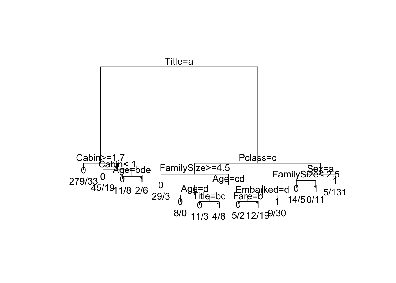
plot(dt_prune, margin = 0.1)
text(dt_prune, use.n = T)
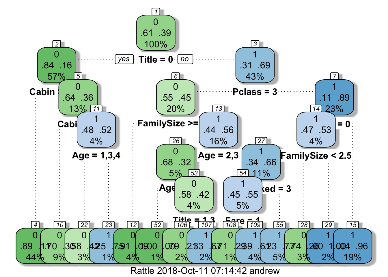
fancyRpartPlot(dt_prune, cex = 1) #fancy tree
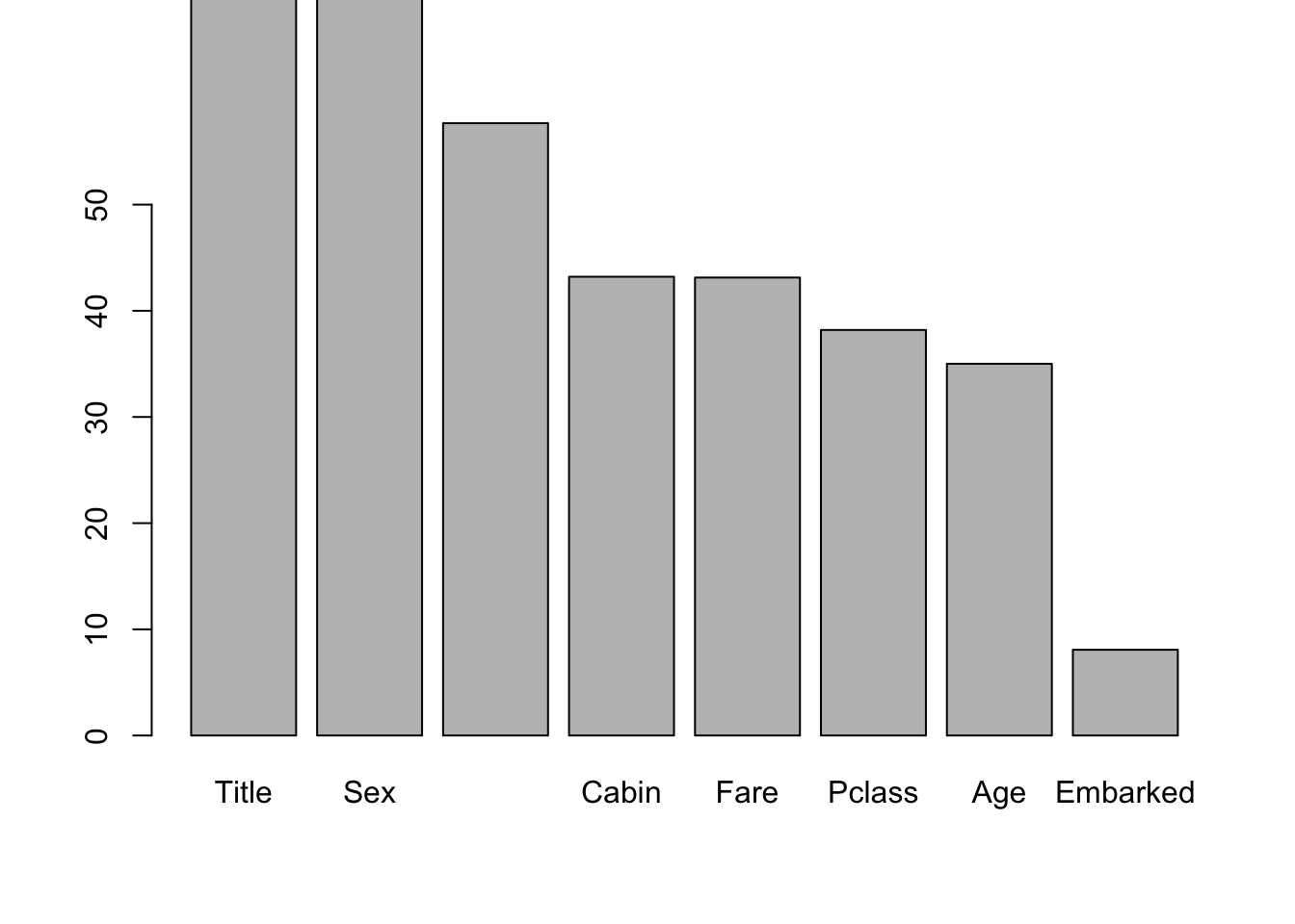
8.2. Feature Importance (변수 중요도 파악)
dt_prune$variable.importance
##      Title        Sex FamilySize      Cabin       Fare     Pclass
## 106.738246  87.102115  57.672985  43.209328  43.133154  38.195278
##        Age   Embarked
##  35.010839   8.076284
barplot(dt_prune$variable.importance, ylim = c(0, 55))
9. Modeling 3 : Logistic Regression
9.1. 모형 만들기
rmse <- function(yi, yhat_i){
  sqrt(mean((yi - yhat_i)^2))
}

binomial_deviance <- function(y_obs, yhat){
  epsilon = 0.0001
  yhat = ifelse(yhat < epsilon, epsilon, yhat)
  yhat = ifelse(yhat > 1-epsilon, 1-epsilon, yhat)
  a = ifelse(y_obs==0, 0, y_obs * log(y_obs/yhat))
  b = ifelse(y_obs==1, 0, (1-y_obs) * log((1-y_obs)/(1-yhat)))
  return(2*sum(a + b))
}


panel.cor <- function(x, y, digits = 2, prefix = "", cex.cor, ...){
  usr <- par("usr"); on.exit(par(usr))
  par(usr = c(0, 1, 0, 1))
  r <- abs(cor(x, y))
  txt <- format(c(r, 0.123456789), digits = digits)[1]
  txt <- paste0(prefix, txt)
  if(missing(cex.cor)) cex.cor <- 0.8/strwidth(txt)
  text(0.5, 0.5, txt, cex = cex.cor * r)
}
# 로지스틱 회귀모형
data_lm_full <- glm(target_train ~ ., data=train_data, family=binomial)
summary(data_lm_full)
##
## Call:
## glm(formula = target_train ~ ., family = binomial, data = train_data)
##
## Deviance Residuals:
##     Min       1Q   Median       3Q      Max
## -2.3997  -0.6194  -0.3878   0.5710   2.5675
##
## Coefficients:
##             Estimate Std. Error z value Pr(>|z|)
## (Intercept)  11.3433   535.4116   0.021 0.983097
## Pclass2      -1.1244     0.5797  -1.939 0.052443 .
## Pclass3      -2.1968     0.6762  -3.249 0.001158 **
## Sex1          0.7625     0.7918   0.963 0.335553
## Age1         -1.2457     0.4101  -3.037 0.002386 **
## Age2         -1.4878     0.4391  -3.388 0.000704 ***
## Age3         -2.1964     0.4713  -4.661 3.15e-06 ***
## Age4         -2.4793     0.9652  -2.569 0.010206 *
## Fare1         0.3940     0.3487   1.130 0.258499
## Fare2         0.9164     0.4411   2.077 0.037768 *
## Fare3         1.0013     0.6682   1.499 0.133993
## Cabin         0.3827     0.4377   0.874 0.381955
## Embarked1   -10.1580   535.4114  -0.019 0.984863
## Embarked2   -10.0595   535.4115  -0.019 0.985010
## Embarked3   -10.4941   535.4114  -0.020 0.984362
## Title1        1.8614     0.8650   2.152 0.031402 *
## Title2        3.0670     0.8764   3.499 0.000466 ***
## Title3        1.4962     0.3732   4.010 6.08e-05 ***
## FamilySize   -0.4798     0.1140  -4.210 2.56e-05 ***
## ---
## Signif. codes:  0 '***' 0.001 '**' 0.01 '*' 0.05 '.' 0.1 ' ' 1
##
## (Dispersion parameter for binomial family taken to be 1)
##
##     Null deviance: 952.58  on 711  degrees of freedom
## Residual deviance: 599.99  on 693  degrees of freedom
## AIC: 637.99
##
## Number of Fisher Scoring iterations: 12
anova(data_lm_full)
## Analysis of Deviance Table
##
## Model: binomial, link: logit
##
## Response: target_train
##
## Terms added sequentially (first to last)
##
##
##            Df Deviance Resid. Df Resid. Dev
## NULL                         711     952.58
## Pclass      2   90.066       709     862.52
## Sex         1  194.740       708     667.78
## Age         4   19.765       704     648.01
## Fare        3    1.059       701     646.95
## Cabin       1    0.002       700     646.95
## Embarked    3    5.384       697     641.57
## Title       3   21.026       694     620.54
## FamilySize  1   20.553       693     599.99
predict(data_lm_full, newdata = train_data, type='response') %>% head()
##        456        814        636        631        138        223
## 0.09853743 0.40126602 0.74461004 0.15240488 0.25270805 0.03702682
# table(y_obs, yhat_lm)
9.2. 모형 평가
# 모형평가
y_obs <- as.numeric(target_valid)
yhat_lm <- predict(data_lm_full, newdata = valid_data, type='response')
pred_lm <- prediction(yhat_lm, y_obs)
performance(pred_lm, "auc")@y.values[[1]]
## [1] 0.8639752
binomial_deviance(y_obs, yhat_lm)
## [1] NaN
10. Lasso regression
10.1. 모형 개발
train2 <- train[,-1]
head(train2)
##   Pclass Sex Age Fare Cabin Embarked Title FamilySize
## 1      3   0   1    0   2.0        3     0          2
## 2      1   1   3    2   0.8        1     2          2
## 3      3   1   1    0   2.0        3     1          1
## 4      1   1   2    2   0.8        3     2          2
## 5      3   0   2    0   2.0        3     0          1
## 6      3   0   2    0   2.0        2     0          1
# 라쏘 모형 적합
xx <- model.matrix(target ~ .-1, train2)
x <- xx[training_idx, ]
y <- as.numeric(as.character(target_train))
glimpse(x)
##  num [1:712, 1:19] 0 0 0 1 1 0 1 0 0 0 ...
##  - attr(*, "dimnames")=List of 2
##   ..$ : chr [1:712] "456" "814" "636" "631" ...
##   ..$ : chr [1:19] "Pclass1" "Pclass2" "Pclass3" "Sex1" ...
10.2. 모형 시각화
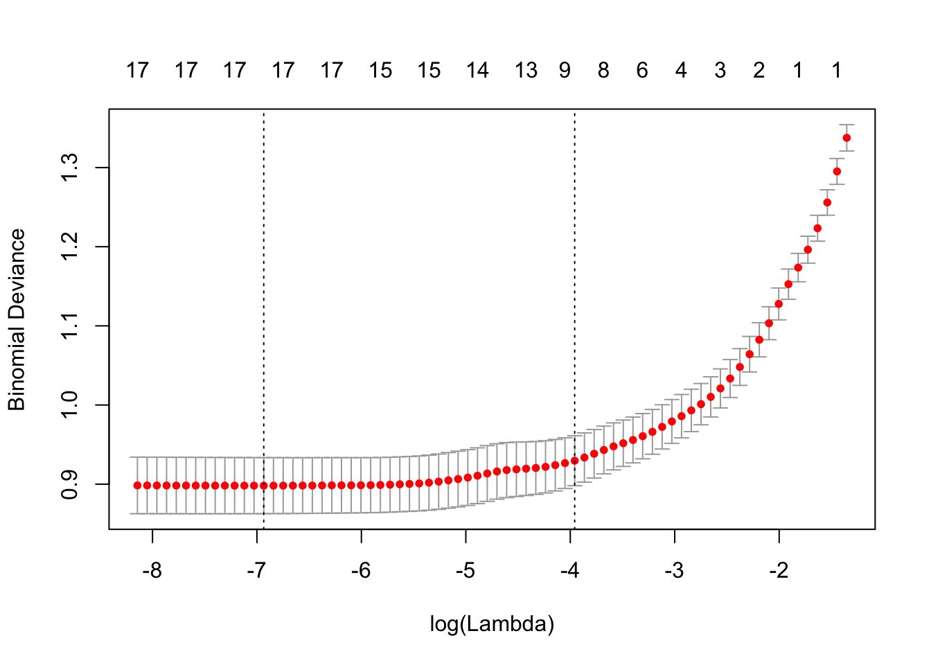
data_cvfit <- cv.glmnet(x, y, family = "binomial")
plot(data_cvfit)
coef(data_cvfit, s = c("lambda.1se"))
## 20 x 1 sparse Matrix of class "dgCMatrix"
##                       1
## (Intercept) -0.87076191
## Pclass1      0.67787153
## Pclass2      .
## Pclass3     -0.91085195
## Sex1         2.26321453
## Age1         .
## Age2         .
## Age3        -0.20513778
## Age4        -0.05129920
## Fare1        .
## Fare2        .
## Fare3        .
## Cabin        .
## Embarked1    .
## Embarked2    .
## Embarked3   -0.20733082
## Title1       .
## Title2       0.29479807
## Title3       0.83763307
## FamilySize  -0.05056563
coef(data_cvfit, s = c("lambda.min"))
## 20 x 1 sparse Matrix of class "dgCMatrix"
##                       1
## (Intercept)  0.16421420
## Pclass1      0.99844117
## Pclass2      .
## Pclass3     -1.03744475
## Sex1         0.89733744
## Age1        -1.08779075
## Age2        -1.31930354
## Age3        -1.98776042
## Age4        -2.26145163
## Fare1        0.31825382
## Fare2        0.79023599
## Fare3        0.82539775
## Cabin        0.22630128
## Embarked1    .
## Embarked2    0.05759651
## Embarked3   -0.33325614
## Title1       1.69603826
## Title2       2.81826506
## Title3       1.44755954
## FamilySize  -0.42835326
10.3. 모형 평가
predict.cv.glmnet(data_cvfit, s="lambda.min", newx = x[1:5,], type='response')
##             1
## 456 0.1026349
## 814 0.4088442
## 636 0.7472538
## 631 0.1762227
## 138 0.2604192
yhat_glmnet <- predict(data_cvfit, s="lambda.min", newx=xx[validate_idx,], type='response')
yhat_glmnet <- yhat_glmnet[,1] # change to a vector from [n*1] matrix
pred_glmnet <- prediction(yhat_glmnet, y_obs)
performance(pred_glmnet, "auc")@y.values[[1]]
## [1] 0.8689441
binomial_deviance(y_obs, yhat_glmnet)
## [1] NaN
11. Boosting
# 부스팅
#set.seed(1607)
#data_for_gbm <-
#  train_data %>%
#  mutate(class=target_train)
#data_gbm <- gbm(target_train ~ ., data=data_for_gbm, distribution="bernoulli",
#              n.trees=50000, cv.folds=3, verbose=TRUE)
#(best_iter = gbm.perf(data_gbm, method="cv"))
# png("../../plots/10-6.png", 5.5, 4, units='in', pointsize=9, res=600)
#(best_iter = gbm.perf(data_gbm, method="cv"))
# dev.off()
#yhat_gbm <- predict(data_gbm, n.trees=best_iter, newdata=validation, type='response')
#pred_gbm <- prediction(yhat_gbm, y_obs)
#performance(pred_gbm, "auc")@y.values[[1]]
#binomial_deviance(y_obs, yhat_gbm)
12. Random Forest
# 랜덤포레스트
set.seed(1607)
data_rf <- randomForest(target_train ~ ., train_data)
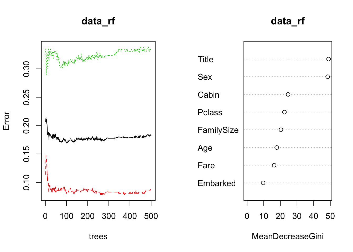
data_rf
##
## Call:
##  randomForest(formula = target_train ~ ., data = train_data)
##                Type of random forest: classification
##                      Number of trees: 500
## No. of variables tried at each split: 2
##
##         OOB estimate of  error rate: 18.26%
## Confusion matrix:
##     0   1 class.error
## 0 396  38   0.0875576
## 1  92 186   0.3309353
opar <- par(mfrow=c(1,2))
plot(data_rf)
varImpPlot(data_rf)
par(opar)
yhat_rf <- predict(data_rf, newdata=valid_data, type='prob')[,'1']
pred_rf <- prediction(yhat_rf, y_obs)
performance(pred_rf, "auc")@y.values[[1]]
## [1] 0.8815045
binomial_deviance(y_obs, yhat_rf)
## [1] NaN
13. 최종 모형선택과 테스트셋 오차계산
# 최종 모형선택과  테스트셋 오차계산
#data.frame(method=c('lm', 'glmnet', 'rf', 'gbm'),
data.frame(method=c('lm', 'glmnet', 'rf'),
           auc = c(performance(pred_lm, "auc")@y.values[[1]],
                   performance(pred_glmnet, "auc")@y.values[[1]],
                   performance(pred_rf, "auc")@y.values[[1]]),
#                   performance(pred_rf, "auc")@y.values[[1]],
#                   performance(pred_gbm, "auc")@y.values[[1]]),
           bin_dev = c(binomial_deviance(y_obs, yhat_lm),
                       binomial_deviance(y_obs, yhat_glmnet),
                       binomial_deviance(y_obs, yhat_rf)))
##   method       auc bin_dev
## 1     lm 0.8639752     NaN
## 2 glmnet 0.8689441     NaN
## 3     rf 0.8815045     NaN
#                       binomial_deviance(y_obs, yhat_rf),
#                       binomial_deviance(y_obs, yhat_gbm)))
# glmnet이 최종 승리자:
##y_obs_test <- as.numeric(as.character(test$class))
##yhat_glmnet_test <- predict(data_cvfit, s="lambda.min", newx=xx[test_idx,], type='response')
##yhat_glmnet_test <- yhat_glmnet_test[,1]
##pred_glmnet_test <- prediction(yhat_glmnet_test, y_obs_test)
##performance(pred_glmnet_test, "auc")@y.values[[1]]
##binomial_deviance(y_obs_test, yhat_glmnet_test)
14. ROC 커브
# 예측값들의 상관관계
# ROC 커브
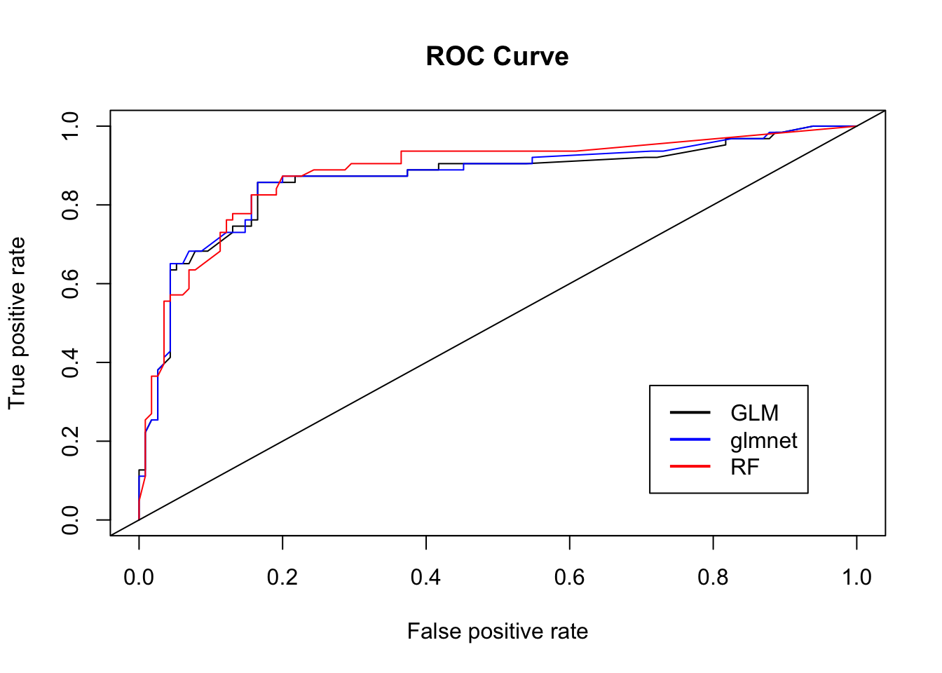
perf_lm <- performance(pred_lm, measure = "tpr", x.measure = "fpr")
perf_glmnet <- performance(pred_glmnet, measure="tpr", x.measure="fpr")
perf_rf <- performance(pred_rf, measure="tpr", x.measure="fpr")
#perf_gbm <- performance(pred_gbm, measure="tpr", x.measure="fpr")
# png("../../plots/10-7.png", 5.5, 4, units='in', pointsize=9, res=600)
plot(perf_lm, col='black', main="ROC Curve")
plot(perf_glmnet, add=TRUE, col='blue')
plot(perf_rf, add=TRUE, col='red')
#plot(perf_gbm, add=TRUE, col='cyan')
abline(0,1)
legend('bottomright', inset=.1,
    legend=c("GLM", "glmnet", "RF"),
    col=c('black', 'blue', 'red'), lty=1, lwd=2)
#    legend=c("GLM", "glmnet", "RF", "GBM"),
#    col=c('black', 'blue', 'red', 'cyan'), lty=1, lwd=2)
# dev.off()
# png("../../plots/10-8.png", 5.5, 4, units='in', pointsize=9, res=600)
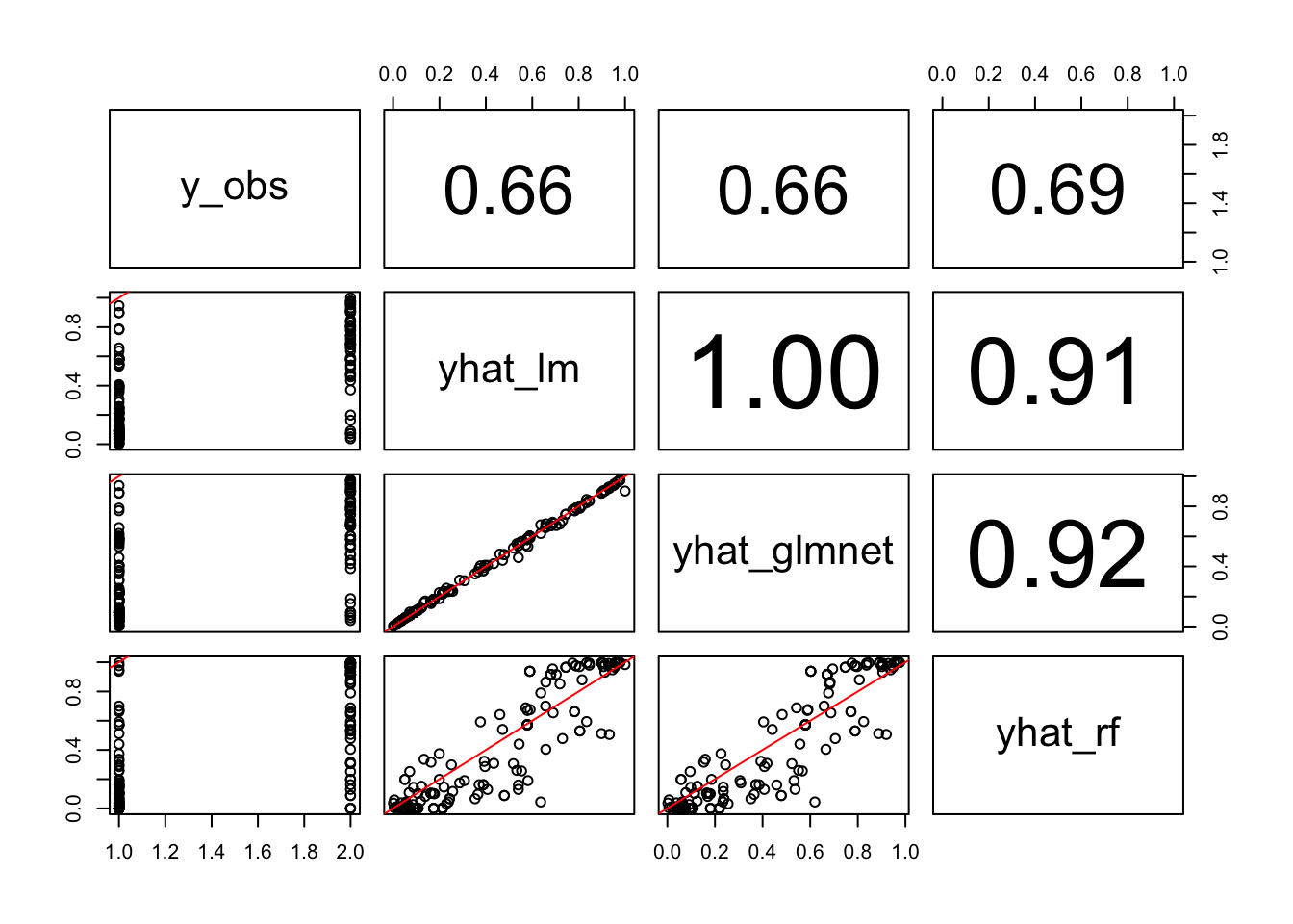
pairs(data.frame(y_obs=y_obs,
                 yhat_lm=yhat_lm,
                 yhat_glmnet=c(yhat_glmnet),
                 yhat_rf=yhat_rf),
#                 yhat_rf=yhat_rf,
#                 yhat_gbm=yhat_gbm),
      lower.panel=function(x,y){ points(x,y); abline(0, 1, col='red')},
      upper.panel = panel.cor)
# dev.off()
# 6. Modelling
## 6.1. Cross Validation (K-fold)

## 6.2. kNN

## 6.3. Decision Tree
## 6.4. Ramdom Forest

## 6.5. Naive Bayes

## 6.6. SVM

# 7. Testing
[출처] https://rstudio-pubs-static.s3.amazonaws.com/425150_0ce41e78ad404451b70a6cd0cfcfe71d.html
광고 클릭에서 발생하는 수익금은 모두 웹사이트 서버의 유지 및 관리, 그리고 기술 콘텐츠 향상을 위해 쓰여집니다.
댓글 0
| 번호 | 제목 | 글쓴이 | 날짜 | 조회 수 |
|---|---|---|---|---|
| 공지 | 오라클 기본 샘플 데이터베이스 | 졸리운_곰 | 2014.01.02 | 88974 |
| 공지 | [SQL컨셉] 서적 "SQL컨셉"의 샘플 데이타 베이스 SAMPLE DATABASE of ORACLE | 가을의 곰을... | 2013.02.10 | 80924 |
| 공지 | [G_SQL] Sample Database | 가을의 곰을... | 2012.05.20 | 97542 |
| 1 | [hadoop] Python으로 Hive 연결하기 | 졸리운_곰 | 2021.03.04 | 1505 |