[러닝 텐서플로]Chap07.1 - 텐서플로 추상화와 간소화, Estimator 

Chap07.1 - 텐서플로 추상화와 간소화, Estimator

추상화가 무엇이며 왜 유용한지 알아보고 텐서플로(TensorFlow)의 몇몇 대중적인 추상화 라이브러리를 간단하게 살펴보도록 하자.

 

7.1 개요

추상화(abstraction)이란 코드를 특정한 목적으로 일반화하여 기존 코드 '위에 올라가는' 코드의 계층을 의미한다. 관련있는 High-Level 기능을 묶는 방식의 재구성을 통해 코드를 감싸서 추상화한다. 따라서 쉽게 코딩할 수 있고, 가독성이 좋으며, 코드가 간소화된다.

 

7.1.1 추상화 라이브러리 둘러보기

텐서플로(TensorFlow)에서 사용할 수 있는 인기있는 추상화 라이브러리는 다음과 같다고 한다.

• tf.estimator

• TFLearn

• TF-Slim

• Keras

TFLearn은 별도의 설치가 필요하며 tf.estimator과 TF-Slim(tf.contrib.slim)은 텐서플로에 포함되어 있다. Keras(케라스)는 2017년 구글의 공식 후원을 받아 1.1버전 부터 tf.contrib.keras안에 들어왔으며, 현재 이글을 작성하는 시점인 2018.06.27의 1.8버전에는 tf.keras로 변경됭 텐서플로의 한 부분으로 자리를 잡았다. contrib안의 라이브러리들은 기부된(contributed) 것을 의미하며 정식으로 반영되기 전까지 테스트가 더 필요하다는 것을 의미한다.

tf.estimator은 Python의 대표적인 머신러닝 모듈인 Scikit-Learn(sklearn)의 스타일처럼 복잡한 딥러닝 모델을 쉽게 작성할 수 있도록 해주는 라이브러리다. Keras와 마찬가지로 tf.contrib.learn으로 텐서플로에 들어왔으며, 현재 1.8버전(2018.06.27)에는 tf.estimator로 옮겨졌으며 tf.contrib.learn은 유지되고 있지만 사용할 경우 deprecated 경고가 나타난다.

TF-Slim은 주로 복잡한 합성곱 신경망(Convolutional Networks)을 쉽게 설계할 수 있도록 만들어졌으며 다양한 Pre-Trained 모델을 제공해 학습 시간을 단축시킬 수 있다.

 

7.2 tf.estimator

tf.estimator는 sklearn과 유사하게 Estimator(모델들을 부르는 용어)로 동작하는데 이것을 이용하면, 빠르게 모델을 학습할 수 있다. 대표적인 Estimator들은 아래와 같으며, tf.estimator에서 다양한 Estimator들을 살펴볼 수 있다.

 

 

Estimator	설명
LinearRegressor()	주어진 관측치에 대해 Linear regression을 이용해 예측
LinearClassifier()	Linear Model을 이용한 다중분류(multi-classification), 클래스가 2개일 경우 binary classification
DNNRegressor()	TensorFlow DNN 모델을 이용한 regression
DNNClassifier()	TensorFlow DNN 모델을 이용한 classification

tf.contrib.learn에서 tf.estimator로 옮겨올때 아래의 Estimator는 반영이 되지 않았다.

• DynamicRnnEstimator: Consider a custom model_fn.

• KMeansClustering: Use tf.contrib.factorization.KMeansClustering.

• LogisticRegressor: Not supported. Instead, use binary_classification_head with a custom model_fn, or with DNNEstimator.

• StateSavingRnnEstimator: Consider a custom model_fn.

• SVM: Consider a custom model_fn.

• LinearComposableModel and DNNComposableModel: Not supported. Consider tf.contrib.estimator.DNNEstimator, or write a custom model_fn.

• MetricSpec: Deprecated. For adding custom metrics to canned Estimators, use tf.contrib.estimator.add_metrics.

위의 Estimator를 사용하는 방법은 다음과 같다.

1. 클래스 인스턴스화(instance)

   • model = tf.estimator.<some_Estimator>()

2. 학습 데이터를 사용해 모델을 학습

   • model.train()

3. 학습된 모델을 평가(evaluate)

   • model.evaluate()

4. 테스트 데이터를 이용해 결과를 예측(predict)

   • model.predict()

 

 

7.2.1 선형회귀 - Linear Regression

선형회귀(linear regression)은 데이터 집합 ​ 에 대해, 종속변수 ​와 ​개의 설명변수 ​ 사이의 선형 관계를 모델링한다(출처: wikipedia).

 

 

위의 선형회귀 모델을 Scikit-Learn(사이킷런)에서 제공하는 보스턴 하우징(Boston Housing)데이터에 적용해보도록 하자. 먼저 추상화 라이브러리를 사용하지 않은 텐서플로(TensorFlow)코드를 구현한 뒤, 이것을 tf.estimator.LiearRegressor()를 이용해 구현해 볼 것이다.

보스턴 하우징 데이터 설명은 다음과 같다. 종속변수(타겟변수)는 소유자가 거주 중인 주택 가격의 중간값(median)이다.

 

	Feature	설명
1	CRIM	마을의 1인당 범죄율
2	ZN	2만 5천 평방 피트 이상으로 구획된 택지의 비율
3	INDUS	마을당 비상업 업무 지구의 비율
4	CHAS	찰스강 더미 변수 (인접: 1, 아니면: 0)
5	NOX	질소산화물 농도
6	RM	주택당 평균 방의 수
7	AGE	1940년 이전에 지어진 건물의 비율
8	DIS	5개의 보스턴 고용 센터까지의 가중 거리
9	RAD	방사형 고속도로까지의 접근성 지수
10	TAX	1만 달러당 부가가치세
11	PTRATIO	마을별 학생 대 교사 비율
12	B	​, ​: 마을의 흑인 비율
13	LSTAT	하위 계층의 비율(%)

먼저 Scikit-Learn에서 보스턴 하우징 데이터를 불러온다. 설명변수로 쓰일 데이터들을 StandardScaler()를 이용해 정규화 해준다. StandardScaler의 수식은 다음과 같으며 Z-Score라고도 한다.

 

 

 

 

from sklearn import datasets, metrics, preprocessing
​
boston = datasets.load_boston()
x_data = preprocessing.StandardScaler().fit_transform(boston.data)
y_data = boston.target
​
print('x_data.shape :', x_data.shape)
print('y_data.shape :', y_data.shape)

 

x_data.shape : (506, 13)
y_data.shape : (506,)

 

 

Natvie TensorFlow

먼저 추상화 라이브러리를 사용하지 않고, 순수 텐서플로를 이용해 선형회귀를 모델링 해보도록 하자.

 

import tensorflow as tf

 

x = tf.placeholder(tf.float64, shape=(None, 13))
y_true = tf.placeholder(tf.float64, shape=(None))
​
with tf.name_scope('inference'):
   w = tf.Variable(tf.zeros([1, 13], dtype=tf.float64, name='weights'))
   b = tf.Variable(0, dtype=tf.float64, name='bias')
   y_pred = tf.matmul(w, tf.transpose(x)) + b
   
with tf.name_scope('loss'):
   loss = tf.reduce_mean(tf.square(y_true-y_pred))  # MSE
   
with tf.name_scope('train'):
   learning_rate = 0.1
   optimizer = tf.train.GradientDescentOptimizer(learning_rate)
   train = optimizer.minimize(loss)
   
init = tf.global_variables_initializer()
with tf.Session() as sess:
   sess.run(init)
   for step in range(200):
       MSE, _ = sess.run([loss, train], feed_dict={x: x_data, 
                                                   y_true: y_data})
   
       if (step+1) % 40 == 0:
           print('Step: {:2d}\t MSE: {:.5f}'.format(step+1, MSE))

 

Step: 40 MSE: 22.30192
Step: 80 MSE: 22.00200
Step: 120 MSE: 21.93284
Step: 160 MSE: 21.91024
Step: 200 MSE: 21.90225

 

 

tf.estimator

이번에는 위와 똑같은 기능을 하는 코드를 tf.estimator.LinearRegressor()를 이용해 구현해 보도록 하자. 아래의 코드에서 확인할 수 있듯이 간단한 코드로 Linear Regression을 구현할 수 있다.

 

NUM_STEPS = 200
MINIBATCH_SIZE = 506
​
feature_column = [tf.feature_column.numeric_column(key='x', shape=13)]
train_input_fn = tf.estimator.inputs.numpy_input_fn(
      {'x': x_data}, y_data, batch_size=MINIBATCH_SIZE, shuffle=False)
eval_input_fn = tf.estimator.inputs.numpy_input_fn(
      {'x': x_data}, y_data, batch_size=MINIBATCH_SIZE, shuffle=False)
​
reg = tf.estimator.LinearRegressor(
       feature_columns=feature_column,
       optimizer=tf.train.GradientDescentOptimizer(learning_rate=0.001), 
       model_dir='./model/boston')
​
reg.train(input_fn=train_input_fn, steps=NUM_STEPS)
MSE = reg.evaluate(input_fn=eval_input_fn, steps=1)
​
print(MSE)

 

 

 

7.2.2 DNN 분류기

이번에는 2.4 - Softmax Regression에서 구현한 MNIST 분류기를 tf.estimator.DNNClassifier()를 이용해 구현해보도록 하자.

 

import sys
import numpy as np
import tensorflow as tf
​
​
# MNIST 데이터 불러오기 위한 함수 정의
def mnist_load():
  (train_x, train_y), (test_x, test_y) = tf.keras.datasets.mnist.load_data()
​
   # Train set
   train_x = train_x.astype('float32') / 255.
   train_y = train_y.astype('int32')
   # Test set
   test_x = test_x.astype('float32') / 255.
   test_y = test_y.astype('int32')
   return (train_x, train_y), (test_x, test_y)
​
# MNIST 데이터 불러오기
(train_x, train_y), (test_x, test_y) = mnist_load()
​
# Define train_input_fn
train_input_fn = tf.estimator.inputs.numpy_input_fn(
   x={'x': train_x}, y=train_y, shuffle=True, batch_size=MINIBATCH_SIZE
)

 

NUM_STEPS = 5000
MINIBATCH_SIZ = 128
​
feature_columns = [tf.feature_column.numeric_column('x', shape=[28, 28])]
​
dnn = tf.estimator.DNNClassifier(
   feature_columns=feature_columns,
   hidden_units=[200],
   n_classes=10,
   optimizer=tf.train.ProximalAdagradOptimizer(learning_rate=0.2),
   model_dir='./model/DNNClassifier'
)
​
dnn.train(
   input_fn=train_input_fn,
   steps=NUM_STEPS)

 

INFO:tensorflow:Using default config.
INFO:tensorflow:Using config: {'_model_dir': './model', '_tf_random_seed': None, '_save_summary_steps': 100, '_save_checkpoints_steps': None, '_save_checkpoints_secs': 600, '_session_config': None, '_keep_checkpoint_max': 5, '_keep_checkpoint_every_n_hours': 10000, '_log_step_count_steps': 100, '_train_distribute': None, '_service': None, '_cluster_spec': <tensorflow.python.training.server_lib.ClusterSpec object at 0x7f0bca1f3908>, '_task_type': 'worker', '_task_id': 0, '_global_id_in_cluster': 0, '_master': '', '_evaluation_master': '', '_is_chief': True, '_num_ps_replicas': 0, '_num_worker_replicas': 1}
INFO:tensorflow:Calling model_fn.
INFO:tensorflow:Done calling model_fn.
INFO:tensorflow:Create CheckpointSaverHook.
INFO:tensorflow:Graph was finalized.
INFO:tensorflow:Running local_init_op.
INFO:tensorflow:Done running local_init_op.
INFO:tensorflow:Saving checkpoints for 1 into ./model/model.ckpt.
INFO:tensorflow:loss = 1178.339, step = 0
INFO:tensorflow:global_step/sec: 298.774
INFO:tensorflow:loss = 121.545364, step = 100 (0.336 sec)
INFO:tensorflow:Saving checkpoints for 119 into ./model/model.ckpt.
INFO:tensorflow:Loss for final step: 95.376915.

 

# Define eval_input_fn
eval_input_fn = tf.estimator.inputs.numpy_input_fn(
   x={'x': test_x}, y=test_y, shuffle=False
)
​
test_acc = dnn.evaluate(input_fn=eval_input_fn, steps=1)['accuracy']
print('test accuracy: {}'.format(test_acc))

 

INFO:tensorflow:Calling model_fn.
INFO:tensorflow:Done calling model_fn.
INFO:tensorflow:Starting evaluation at 2018-06-27-10:03:23
INFO:tensorflow:Graph was finalized.
INFO:tensorflow:Restoring parameters from ./model/model.ckpt-119
INFO:tensorflow:Running local_init_op.
INFO:tensorflow:Done running local_init_op.
INFO:tensorflow:Evaluation [1/1]
INFO:tensorflow:Finished evaluation at 2018-06-27-10:03:23
INFO:tensorflow:Saving dict for global step 119: accuracy = 0.9453125, average_loss = 0.2138238, global_step = 119, loss = 27.369446
test accuracy: 0.9453125

 

 

7.2.3 tf.feature_column

텐서플로는 tf.feature_column를 통해 다양한 데이터의 특징(Feature)들을 처리해준다. 7.2.1과 7.2.2에서 tf.estimator를 이용해 Estimator를 만들어줄때 tf.feature_column.numeric_column()를 이용해서 데이터의 특징(feature)을 정의해줬다.

이렇듯 수치형 데이터도 있지만, 실제 세계에서는 아래의 예시(출처: TensorFlow.org)와 같이 수치형 데이터 뿐만 아니라 다양한 특징(특성)들을 가지는 데이터들이 존재한다.

 

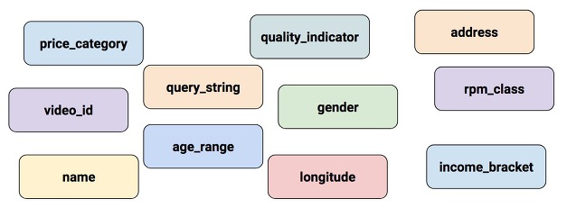
tf.feature_column이 제공하는 특징 처리 중 몇가지 예로는 범주형(categorical) 데이터를 희소 벡터, 즉 one-hot 인코딩(또는 더미 인코딩, dummy encoding)해주며, 또는 수치형 데이터를 구간별로 버킷화(bucketize)한 뒤 더미 인코딩 해준다. 이 외에도 다양한 특징들을 처리해주는데 자세한 내용은 TensorFlow.org에서 확인할 수 있다.

tf.feature_column은 크게 CategoricalColumn과 DenseColumn으로 이루어져 있으며 이 둘을 동시에 상속받는 bucketized_column이 있다.(출처: TensorFlow.org)

 

그렇다면, 이러한 tf.feature_column을 어떻게 사용하는지 간단한 샘플 데이터로 사용법을 알아보도록 하자.

예를 들어, 무게(weight)와 종족(species) 두 개의 특징(feature)으로 타겟변수인 키(height)를 tf.estimator.LinearRegressor()를 이용해 예측한다고 가정해보자. 각 무게를 100으로 나누고 종(species)에 따른 상수(Human=1, Goblin=0.98, ManBear=1.1) 을 추가해 샘플 데이터를 아래의 코드와 같이 만들어준다.

 

# Generate example categorical data
import numpy as np
import pandas as pd
​
N = 10000
weight = np.random.randn(N)*5 + 70
spec_id = np.random.randint(0, 3, N)
bias = [0.9, 1, 1.1]
height = np.array([weight[i]/100 + bias[b] for i, b in enumerate(spec_id)])
spec_name = ['Goblin', 'Human', 'ManBears']
spec = [spec_name[s] for s in spec_id]

 

생성한 예제 샘플 데이터를 matplotlib을 이용해 시각화 해보자.

 

# plot and create data frame
%matplotlib inline
import matplotlib.pyplot as plt
​
colors = ['r','b','g']
f,axarr = plt.subplots(1,2,figsize = [7,3])
ax = axarr[0]
for ii in range(3):
   ax.hist(height[spec_id == ii],50,color=colors[ii],alpha=0.5)
   ax.set_xlabel('Height')
   ax.set_ylabel('Frequency')
   ax.set_title('Heights distribution')
​
height = height + np.random.randn(N)*0.015
ax.text(1.42,150,'Goblins')
ax.text(1.63,210,'Humans')
ax.text(1.85,150,'ManBears')
​
ax.set_ylim([0,260])
ax.set_xlim([1.38,2.05])
​
df = pd.DataFrame({'Species':spec,'Weight':weight,'Height':height})
​
ax = axarr[1]
ax.plot(df['Height'],df['Weight'],'o',alpha=0.3,mfc='w',mec='b')
ax.set_xlabel('Weight')
ax.set_ylabel('Height')
ax.set_title('Heights vs. Weights')
   
plt.tight_layout()
plt.show()

 

 

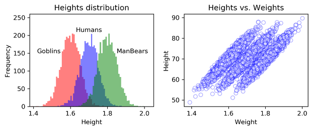
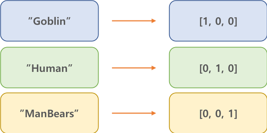
이제, LinearRegressor()의 입력(Input)으로 넣어주기 위해 tf.feature_column을 이용해 각 변수의 특성을 지정해준다. Weight는 몸무게이므로 연속형 변수임을 지정하는 numeric_column()을 사용한다. Species는 범주형(categorical) 변수이고, 값이 단어(vocabulary)로 구성되어 있으므로 categorical_column_with_vocabulary_list()를 사용해 특성을 지정해준다. 따라서, 변주형 변수인 Species는 아래의 그림처럼 데이터가 one-hot 벡터로 매핑된다.

 

이렇게 처리된 FeatureColumn들을 LinearRegressor()의 feature_columns=인자에 리스트 형태로 넣어준다.

 

import tensorflow as tf
​
# Feature Columns
Weight = tf.feature_column.numeric_column(key='Weight')
Species = tf.feature_column.categorical_column_with_vocabulary_list(
           key='Species',
           vocabulary_list=['Goblin', 'Human', 'ManBears'])
​
# LinearRegressor() Estimator
reg = tf.estimator.LinearRegressor(feature_columns=[Weight, Species], 
                                  model_dir='./model/sample')

 

위에서 정의한 LinearRegressor()를 학습시킬때(reg.train()) input_fn인자에 학습에 사용할 데이터를 반환하는 캡슐화된 입력함수를 별도로 만들어줘야 한다. 아래의 코드에서 input_fn이 입력함수에 해당하며, pandas의 DataFrame을 입력으로 받아 텐서플로에서 사용가능한 텐서가 들어있는 feature_cols 딕셔너리와 labels을 반환한다.

feature_cols 딕셔너리에서 Species의 값은 위에서 tf.feature_column을 이용해 더미 인코딩을 해주었으므로 이러한 형태를 담을 수 있는 tf.SparseTensor를 사용한다. tf.SparseTensor()는 아래의 예제와 같이 텐서(tensor)의 인덱스에 해당하는 값을 매핑해준다.

 

tf.SparseTensor(indices=[[0, 0], [1, 2]], values=[1, 2], dense_shape=[3, 4])
# 결과
[[1, 0, 0, 0]
[0, 0, 2, 0]
[0, 0, 0, 0]]

 

def input_fn(df):
   feature_cols = {
       'Weight': tf.constant(df['Weight'].values),
       'Species': tf.SparseTensor(
           indices=[[i, 0] for i in range(df['Species'].size)],
           values=df['Species'].values,
           dense_shape=[df['Species'].size, 1]
      )
  }
   labels = tf.constant(df['Height'].values)
   
   return feature_cols, labels
​
# Training
reg.train(input_fn=lambda: input_fn(df), steps=500)

 

학습이 끝난 후 추정된 가중치들을 .get_variable_value()메소드를 이용해 변수의 값을 확인할 수 있다. 변수의 값은 .get_variable_names()를 통해 구할 수 있다.

 

print('variable names:\n', reg.get_variable_names())
print('='*50)
​
w_w = reg.get_variable_value('linear/linear_model/Weight/weights')
s_w = reg.get_variable_value('linear/linear_model/Species/weights')
b = reg.get_variable_value('linear/linear_model/bias_weights')
print('Estimation for Weight: {}'.format(w_w))
print('Estimation for Species:\n{}'.format(s_w + b))

 

variable names:
['global_step', 'linear/linear_model/Species/weights', 'linear/linear_model/Species/weights/part_0/Ftrl', 'linear/linear_model/Species/weights/part_0/Ftrl_1', 'linear/linear_model/Weight/weights', 'linear/linear_model/Weight/weights/part_0/Ftrl', 'linear/linear_model/Weight/weights/part_0/Ftrl_1', 'linear/linear_model/bias_weights', 'linear/linear_model/bias_weights/part_0/Ftrl', 'linear/linear_model/bias_weights/part_0/Ftrl_1']
==================================================
Estimation for Weight: [[0.01007662]]
Estimation for Species:
[[0.8940179]
[0.9947232]
[1.0953919]]

 

 

7.2.4 tf.estimator로 사용자 정의 CNN 만들어보기

이번에는 tf.estimator를 사용해 자신만의 Estimator를 만들어 보자. 아래의 예제 코드는 4장-합성곱 신경망 CNN에서와 마찬가지로 MNIST 데이터 분류를 tf.estimator를 이용해 구현해 보도록한다.먼저 네트워크를 구현하는 모델 함수(cnn_model_fn)와 학습 설정(model_params)을 포함한 객체를 만들어줘야 한다. 아래의 코드는 TensorFlow.org의 Tutorials를 참고하여 구현하였다.

 

# model_params
model_params = {"learning_rate": 1e-4, "dropout": 0.5}
​
# Generate model_fn
def cnn_model_fn(features, labels, mode, params):
   # Input Layer
   x_image = tf.reshape(features['x'], [-1, 28, 28, 1])  # (N, H, W, C)
   
   # Conv layer 1
   conv1 = tf.layers.conv2d(x_image, 32, [5,5],
                            padding='same',
                            activation=tf.nn.relu,
                            kernel_initializer=tf.truncated_normal_initializer(stddev=0.1),
                            bias_initializer=tf.constant_initializer(0.1))
   pool1 = tf.layers.max_pooling2d(conv1, pool_size=[2,2], strides=2)
   
   # Conv layer 2
   conv2 = tf.layers.conv2d(pool1, 64, [5,5],
                            activation=tf.nn.relu,
                            padding='same',
                            kernel_initializer=tf.truncated_normal_initializer(stddev=0.1),
                            bias_initializer=tf.constant_initializer(0.1))
   pool2 = tf.layers.max_pooling2d(conv2, pool_size=[2,2], strides=2)
   
   # Fully-Connected layer
   pool2_flat = tf.reshape(pool2, [-1, 7*7*64])
   dense = tf.layers.dense(pool2_flat, 1024,
                         activation=tf.nn.relu,
                         kernel_initializer=tf.truncated_normal_initializer(stddev=0.1),
                         bias_initializer=tf.constant_initializer(0.1))
   dropout = tf.layers.dropout(dense, 
                               rate=params['dropout'],  # rate: dropout 시킬 비율
                               training=mode == tf.estimator.ModeKeys.TRAIN)
   
   # Logits layer
   logits = tf.layers.dense(dropout, 10, activation=None)
   
    # prediction
   predictions = {
       # Generate predictions (for PREDICT and EVAL mode)
       "classes": tf.argmax(input=logits, axis=1)
  }
   
   if mode == tf.estimator.ModeKeys.PREDICT:
       return tf.estimator.EstimatorSpec(mode=mode, predictions=predictions)
   
   # loss (for both TRAIN and EVAL modes)
   loss = tf.losses.sparse_softmax_cross_entropy(logits=logits, labels=labels)
   
   # Configure the Training Op (for TRIAIN mode)
   if mode == tf.estimator.ModeKeys.TRAIN:
       optimizer = tf.train.AdamOptimizer(learning_rate=params['learning_rate'])
       train_op = optimizer.minimize(loss=loss,
                                     global_step=tf.train.get_global_step())
       return tf.estimator.EstimatorSpec(mode=mode, loss=loss, train_op=train_op)
   
   # Add evaluation metrics (for EVAL mode)
   eval_metric_ops = {
       "accuracy": tf.metrics.accuracy(labels=labels, 
                                       predictions=predictions['classes'])}
   return tf.estimator.EstimatorSpec(mode=mode, loss=loss, 
                                     eval_metric_ops=eval_metric_ops)

 

아래의 코드는 MNIST 데이터를 불러오기 위한 mnist_load()함수를 정의해주고 MNIST 데이터를 불러오는 코드이다.

 

# MNIST 데이터 불러오기 위한 함수 정의
def mnist_load():
  (train_x, train_y), (test_x, test_y) = tf.keras.datasets.mnist.load_data()
​
   # Train set
   train_x = train_x.astype('float32') / 255.
   train_y = train_y.astype('int32')
   # Test set
   test_x = test_x.astype('float32') / 255.
   test_y = test_y.astype('int32')
   return (train_x, train_y), (test_x, test_y)
​
# MNIST 데이터 불러오기
(train_x, train_y), (test_x, test_y) = mnist_load()

 

모델 함수(cnn_model_fn)와 학습 설정(model_params)를 만들었으니, 이제 tf.estimator를 이용해 Estimator를 인스턴스화 해준다.

 

# Generate Estimator
CNN = tf.estimator.Estimator(model_fn=cnn_model_fn,
                            params=model_params,
                            model_dir='./model/mnist_cnn')
​
# Train the model
train_input_fn = tf.estimator.inputs.numpy_input_fn(
       x={'x': train_x},
       y=train_y,
       batch_size=100,
       num_epochs=None,
       shuffle=True)
​
CNN.train(input_fn=train_input_fn, 
         steps=1000)

 

INFO:tensorflow:Using default config.
INFO:tensorflow:Using config: {'_model_dir': './model/mnist_cnn', '_tf_random_seed': None, '_save_summary_steps': 100, '_save_checkpoints_steps': None, '_save_checkpoints_secs': 600, '_session_config': None, '_keep_checkpoint_max': 5, '_keep_checkpoint_every_n_hours': 10000, '_log_step_count_steps': 100, '_train_distribute': None, '_service': None, '_cluster_spec': <tensorflow.python.training.server_lib.ClusterSpec object at 0x00000293A61A8B00>, '_task_type': 'worker', '_task_id': 0, '_global_id_in_cluster': 0, '_master': '', '_evaluation_master': '', '_is_chief': True, '_num_ps_replicas': 0, '_num_worker_replicas': 1}
INFO:tensorflow:Calling model_fn.
INFO:tensorflow:Done calling model_fn.
INFO:tensorflow:Create CheckpointSaverHook.
INFO:tensorflow:Graph was finalized.
INFO:tensorflow:Restoring parameters from ./model/mnist_cnn\model.ckpt-100
INFO:tensorflow:Running local_init_op.
INFO:tensorflow:Done running local_init_op.
INFO:tensorflow:Saving checkpoints for 101 into ./model/mnist_cnn\model.ckpt.
INFO:tensorflow:loss = 0.6972733, step = 101
INFO:tensorflow:global_step/sec: 7.69614
INFO:tensorflow:loss = 0.283104, step = 201 (12.994 sec)
INFO:tensorflow:global_step/sec: 7.50332
INFO:tensorflow:loss = 0.28233457, step = 301 (13.328 sec)
INFO:tensorflow:global_step/sec: 7.82044
INFO:tensorflow:loss = 0.29857188, step = 401 (12.786 sec)
INFO:tensorflow:global_step/sec: 7.8225
INFO:tensorflow:loss = 0.43387017, step = 501 (12.785 sec)
INFO:tensorflow:global_step/sec: 7.77775
INFO:tensorflow:loss = 0.1938857, step = 601 (12.874 sec)
INFO:tensorflow:global_step/sec: 7.36151
INFO:tensorflow:loss = 0.20216578, step = 701 (13.566 sec)
INFO:tensorflow:global_step/sec: 7.56821
INFO:tensorflow:loss = 0.13423444, step = 801 (13.213 sec)
INFO:tensorflow:global_step/sec: 7.65595
INFO:tensorflow:loss = 0.2598955, step = 901 (13.062 sec)
INFO:tensorflow:global_step/sec: 7.78321
INFO:tensorflow:loss = 0.078527495, step = 1001 (12.849 sec)
INFO:tensorflow:Saving checkpoints for 1100 into ./model/mnist_cnn\model.ckpt.
INFO:tensorflow:Loss for final step: 0.14019911.

 

학습이 끝났으면, 테스트 데이터를 이용해 모델을 평가해보자. 아래의 코드는 학습된 Estimator를 .evaluate()를 이용해 Estimator를 평가하는 코드이다.

 

# Evaluate the model and print results
eval_input_fn = tf.estimator.inputs.numpy_input_fn(
       x={'x': test_x},
       y=test_y,
       num_epochs=1,
       shuffle=False)
eval_results = CNN.evaluate(input_fn=eval_input_fn)
print(eval_results)

 

INFO:tensorflow:Calling model_fn.
INFO:tensorflow:Done calling model_fn.
INFO:tensorflow:Starting evaluation at 2018-06-29-02:35:28
INFO:tensorflow:Graph was finalized.
INFO:tensorflow:Restoring parameters from ./model/mnist_cnn\model.ckpt-1100
INFO:tensorflow:Running local_init_op.
INFO:tensorflow:Done running local_init_op.
INFO:tensorflow:Finished evaluation at 2018-06-29-02:35:33
INFO:tensorflow:Saving dict for global step 1100: accuracy = 0.9739, global_step = 1100, loss = 0.0923978
{'accuracy': 0.9739, 'loss': 0.0923978, 'global_step': 1100}

 

 

7.2.5 정리

지금까지 tf.estimator를 이용해 모델을 구현해 보았다. 확실히 Low-Level 텐서플로를 이용해 모델을 학습시키는 부분의 코드 수가 많이 줄어든 것을 확인할 수 있다.

 

tf.estimator에 대한 더 많은 튜토리얼은 https://www.tensorflow.org/tutorials/ 에서 살펴볼 수 있다.

출처: https://excelsior-cjh.tistory.com/157?category=940399 [EXCELSIOR]