If AI is the new electricity, what better time to learn about this new technology than now? One practical way to practice your AI and Machine Learning skills are challenges on kaggle.com. However, jumping straight into the complex problems posted there can be quite daunting at the start. In this blog post, I will share my progress from an empty Python project to a working model to make at least decent predictions.

The Challenge

Of the active competitions on kaggle at the time, https://www.kaggle.com/c/LANL-Earthquake-Prediction/ caught my eye the most. The goal of this challenge is to predict experimental earthquakes based on a series of input voltages, representing the seismic activity at the time. It can, therefore, be categorized as a Time series problem. Learn more about this challenge on the discussion page on kaggle.
You can find the source code for this project on my github page.

Analysing the Data

The first step of any Machine Learning challenge is analyzing the given input and expected output data. For this challenge, we are provided a ~9.6 GB large csv tile consisting of 629.145.480 rows and 2 columns: acoustic_data and time_to_failure. Here, the first column is our input or independent variable while the second column contains the value we want to predict, also called the dependent variable:

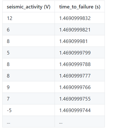
As we can see, the acoustic_data column contains a seemingly random sequence of positive and negative integers while the time_to_failure column consists of floating point values slowly approaching zero. Once it reaches zero, an actual earthquake occurs.

In the test data, we have only an acoustic_data column and have to predict the final time_to_failure after the last input value.

Before we dive into any Machine Learning algorithms, let’s visualize our data. We can do this easily using pandas to load our data and matplotlib for visualization:

import numpy as np
import pandas as pd
import matplotlib.pyplot as plt

data = pd.read_csv('../data/train.csv', 
       dtype={'acoustic_data': np.float32, 'time_to_failure': np.float64})
step = 1000

figure, axis1 = plt.subplots()
x_axis = np.arange(0, len(data), step)
save_plot_data
axis1.plot(x_axis, data.iloc[:, 0][0::step], '-b')
axis1.set_ylabel('sequence')
axis1.set_ylabel('seismic activity', color='b')

axis2 = axis1.twinx()
axis2.plot(x_axis, data.iloc[:, 1][0::step], '-r')
axis2.set_ylabel('time to failure', color='r')

plt.show()

I used a step variable to reduce the number of points matplotlib has to draw. With step set to 1000, we will add only every 1000^th point of the raw data to the plot.
Note that this code will take up to 10GB of your RAM, so if you are working on an older machine, you will probably have to load the data in chunks.
Calling plt.show() gives us the following nice diagram:

From this diagram, we can see that the seismic_activity column reaches values from around -1500 up to +2000 while the time_to_failure goes from 16s down to 0s. By counting how many times the red line reaches 0, we can see that there are in total 16 experimental earthquakes in the training data. It also looks like there is a spike in activity a few seconds before every earthquake.

Feature Engineering

Before we can implement any fancy neural networks or regression models, we have to think about what features we can extract from this dataset. This way, our prediction algorithm won’t have to deal with more than 600 million lines of input and can instead use aggregated values like the mean and standard deviation, quantiles, min and max values, Hilbert transformations, rolling features and many more. Numpy makes extracting such features very straight forward:

def append_features(index: int, stat_summary: pd.core.frame.DataFrame, 
                    step_data: pd.core.frame.DataFrame):
    stat_summary.loc[index, 'mean'] = step_data.mean()
    stat_summary.loc[index, 'std'] = step_data.std()
    stat_summary.loc[index, 'min'] = step_data.min()
    stat_summary.loc[index, 'max'] = step_data.max()

    absolutes = np.abs(step_data)

    stat_summary.loc[index, 'abs_mean'] = absolutes.mean()
    stat_summary.loc[index, 'abs_std'] = absolutes.std()
    stat_summary.loc[index, 'abs_min'] = absolutes.min()
    stat_summary.loc[index, 'abs_max'] = absolutes.max()
    ...

This method takes an index, representing the row we are currently creating for our statistical summary model, a stat_summary DataFrame we will write into and a step_data DataFrame representing the raw data we saw above.

We can call this helper method to create a dataset of summary features:

def get_stat_summaries(data: pd.core.frame.DataFrame, aggregate_length: int = 150000):
    size = len(data)
    stat_summary = pd.DataFrame(dtype=np.float64)

    index = 0
    for i in range(0, size, aggregate_length):
        step_data = data[i:i + aggregate_length]
        append_features(index, stat_summary, step_data.iloc[:, 0])
        index += 1

    return stat_summary

Here, we simply iterate over our dataset and pass every 150.000 rows to the helper method created above. I chose 150.000 as default aggregate_length length because our test datasets are in fact also 150.000 rows long and we want to have the same conditions for our training and test data.
Note that I excluded many of the statistical values I extracted from the dataset to keep the code snippets short. To see the whole range of data we can extract, check out the source code or other kernels on kaggle.

Applied to our training data, calling the code described above gives us a csv file like this:

We have now prepared a new training dataset consisting of 4195 rows and 94 columns. Now, of course, that doesn’t mean that all of these columns will be useful for our model, but it’s better to have too much instead of not enough data.

Creating a Model to Make Predictions

Choosing an appropriate algorithm is a critical step of every Machine Learning problem. It is critical therefore, to do some research about possible solutions and then implement and test some of those algorithms. One algorithm that will quickly catch your eye when you search for Time series prediction problems, are Recurrent neural networks (RNN). RNNs allow us to make predictions for sequences of input by ‘memorizing’ previous input parameters inside an LSTM or GRU. Essentially, they allow us to make predictions based on past input parameters.
Other models we could try are different kinds of Support Vector Machines (SVMs), Time delay neural network, LightGBM and XGB.

I decided to start with an LSTM, but it’s a good idea to play around with all of the above-mentioned models.
Now, before you think about adding 50 hidden input layers to your Neural network, let’s keep it simple and start as small as possible. The network I created for this challenge consists of
one LSTM layer, a hidden fully connected layer and one final output layer to make predictions:

경축! 아무것도 안하여 에스천사게임즈가 새로운 모습으로 재오픈 하였습니다.
어린이용이며, 설치가 필요없는 브라우저 게임입니다.
https://s1004games.com

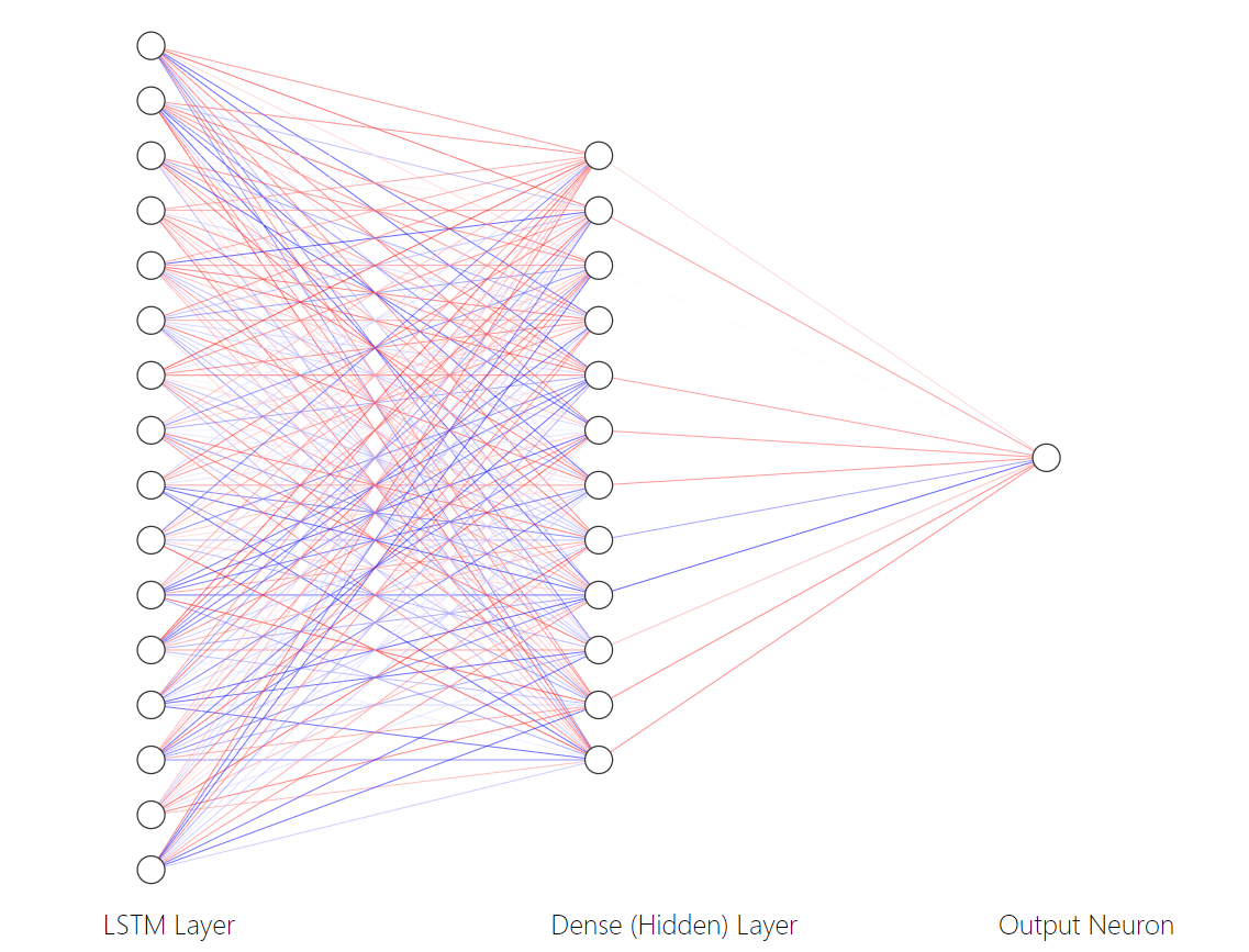
(Created using http://alexlenail.me/NN-SVG/index.html)

One of the easier ways to create RNNs in Python is provided by the Keras API. One way to create RNNs with Keras is to use a CuDNNLSTM layer, a ready to use LSTM implementation.
With that, creating our RNN model is as easy as:

self.model = Sequential()
self.model.add(CuDNNLSTM(64, input_shape=(self.num_features, 1)))
self.model.add(Dense(32, activation='relu'))
self.model.add(Dense(1))   

self.model.compile(optimizer=adam(lr=0.005), loss="mae")

To fit our training data to this neural network, we have to first split up our input dataset into x and y variables. To do so, I created the following helper function:

def _create_x_y(self, data: pd.core.frame.DataFrame):
    x_train, y_train = np.array(data[:, :self.num_features]), np.array(data[:, self.num_features])
    x_train = np.reshape(x_train, (x_train.shape[0], x_train.shape[1], 1))

    return x_train, y_train

Here, we split up our prepared input dataset into two separate numpy arrays and return them.
Using this helper function, we can fit our model with only two more lines of Python code:

x_train, y_train = self._create_x_y(data)
self.model.fit(x_train, y_train, epochs=100, batch_size=64)

This will start the training of our model using 100 epochs and a batch size of 64. After making sure this code works, it’s time to grab a cup of tea and wait for the training to complete (which may take a while depending on your hardware).

Predicting Test Results

Now that our model is trained, it’s time to make use of it to make some predictions. To do so, we have to load the training data and extract all the statistical features from it (like we did for our training data). Then, we can call our RNN model to predict the final time_to_failure of the test dataset. Then, we only have to save these predictions to a CSV file we are going to upload to kaggle later. I implemented all of these steps inside a new helper function:

def predict(model):
    submission = pd.read_csv(
        '../data/sample_submission.csv',
        index_col='seg_id',
        dtype={"time_to_failure": np.float32})

    for i, seg_id in enumerate(submission.index):
        seg = pd.read_csv('../data/test/' + seg_id + '.csv')
        summary = get_stat_summaries(seg, 150000, False)
        submission.time_to_failure[i] = model.predict(summary.values)

    submission.head()
    submission.to_csv('submission.csv')

The predict method is implemented inside our RNN:

def predict(self, x: pd.core.frame.DataFrame):
    x_test = x.reshape(-1, self.num_features)
    scaled = self.scaler.transform(x_test)

    x_test = np.array(scaled[:, :self.num_features])
    x_test = np.reshape(x_test, (x_test.shape[0], x_test.shape[1], 1))

    return self.model.predict(x_test)

Here, we have to apply the same transformations and feature scaling as for our training data. Once this is done, we can call the predict method to get the predicted value based on our test set.

Evaluation

Submitting these predictions on the kaggle submission page, yields an average result of 1.520, which is right in the middleground of all the 600+ predictions from different teams, so there is a lot of space for improvement.
For example, we can try to add more layers to our RNN or to tune some of its many parameters. It would also be useful to apply some feature selection algorithms or try out different statistical values in general.
Cross Validation is another topic not covered by this implementation yet.

Tips for Getting Started on Kaggle

1. Learn From Other Models

Reading and understanding the kernels of other participants in this challenge was probably the most helpful thing to get me started in creating this model. You will see different approaches to solve the given challenge and you will be able to re-use or integrate some of their ideas into your own model.

2. Understanding the Dataset

Try to learn as much as possible about the domain of the problem. How are the input values measured? In what units? Once you understand the problem at hand, it will be easier to come up with creative ways to solve it.

3. Be Ready to Fail

Accept that your models won’t be great in the beginning. Be ready to write a lot of code and throw it away if it doesn’t work out. This is the only way to learn and make progress. As long as you learn something new on your journey, it’s Win-Win! Eventually, your predictions will become better and you will be able to fine-tune your model to make better and better predictions.

4. Have Fun

Most importantly, keep having fun! Machine Learning is one of the most interesting fields in Tech right now, so keep at it even when it gets challenging. If you get frustrated trying to figure out why your model is not working, take a break. Go for a walk, do some sport or get some sleep. Then start again with a fresh mind.