[기계학습] machine learning [기계학습][딥러닝] PyTorch Hello World

2023.02.12 17:02

[기계학습][딥러닝] PyTorch Hello World

I recently started working with PyTorch, a Python framework for neural networks and machine learning. Since machine learning involves processing large amounts of data, sometimes it can be hard to understand the results that one gets back from the network. Before getting into anything more complicated, let’s replicate a really basic backpropagation as a sanity check. To run the code in this article, you’ll need to install NumPy and PyTorch.

In neural networks primer, we saw how to manually calculate the forward and back propagation for a tiny network consisting of one input neuron, one hidden neuron, and one output neuron:

Sample calculation

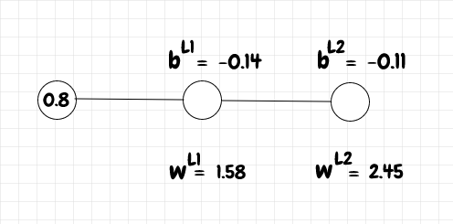
We ran an input of 0.8 through the network, then backpropagated using 1 as the target value, with a learning rate of 0.1. We used sigmoid as the activation function and the quadratic cost function to compare the actual output from the network with the desired output.

The code below uses PyTorch to do the same thing:

import torch
import torch.nn as nn
import torch.optim as optim


class Net(nn.Module):
    def __init__(self):
        super(Net, self).__init__()
        self.hidden_layer = nn.Linear(1, 1)
        self.hidden_layer.weight = torch.nn.Parameter(torch.tensor([[1.58]]))
        self.hidden_layer.bias = torch.nn.Parameter(torch.tensor([-0.14]))

        self.output_layer = nn.Linear(1, 1)
        self.output_layer.weight = torch.nn.Parameter(torch.tensor([[2.45]]))
        self.output_layer.bias = torch.nn.Parameter(torch.tensor([-0.11]))

    def forward(self, x):
        x = torch.sigmoid(self.hidden_layer(x))
        x = torch.sigmoid(self.output_layer(x))
        return x


net = Net()
print(f"network topology: {net}")

print(f"w_l1 = {round(net.hidden_layer.weight.item(), 4)}")
print(f"b_l1 = {round(net.hidden_layer.bias.item(), 4)}")
print(f"w_l2 = {round(net.output_layer.weight.item(), 4)}")
print(f"b_l2 = {round(net.output_layer.bias.item(), 4)}")

# run input data forward through network
input_data = torch.tensor([0.8])
output = net(input_data)
print(f"a_l2 = {round(output.item(), 4)}")

# backpropagate gradient
target = torch.tensor([1.])
criterion = nn.MSELoss()
loss = criterion(output, target)
net.zero_grad()
loss.backward()

# update weights and biases
optimizer = optim.SGD(net.parameters(), lr=0.1)
optimizer.step()

print(f"updated_w_l1 = {round(net.hidden_layer.weight.item(), 4)}")
print(f"updated_b_l1 = {round(net.hidden_layer.bias.item(), 4)}")
print(f"updated_w_l2 = {round(net.output_layer.weight.item(), 4)}")
print(f"updated_b_l2 = {round(net.output_layer.bias.item(), 4)}")

output = net(input_data)
print(f"updated_a_l2 = {round(output.item(), 4)}")

Some notes on this code:

nn.Linear is used for fully connected, or dense, layers. For this simple case, we have a single input and a single output for each layer.
The forward method is called when we pass the input into the network with output = net(input_data).
By default, PyTorch sets up random weights and biases. However, here we initialize them directly since we want the results to match our manual calculation (shown later in the article).
In PyTorch, tensor is analogous to array in numpy.
criterion = nn.MSELoss() sets up the quadratic cost function - though it’s called the mean squared error loss function in PyTorch.
loss = criterion(output, target) calculates the cost, also known as the loss.
Next we use net.zero_grad() to reset the gradient to zero (otherwise the backpropagation is cumulative). It isn’t strictly necessary here, but it’s good to keep this in mind when running backpropagation in a loop.
loss.backward() computes the gradient, i.e. the derivative of the cost with respect to all of the weights and biases.
Finally we use this gradient to update the weights and biases in the network using the SGD (stochastic gradient descent) optimizer, with a learning rate of 0.1.

The results are below:

C:\Dev\python\pytorch>python backprop_pytorch.py
network topology: Net(
  (hidden_layer): Linear(in_features=1, out_features=1, bias=True)
  (output_layer): Linear(in_features=1, out_features=1, bias=True)
)
w_l1 = 1.58
b_l1 = -0.14
w_l2 = 2.45
b_l2 = -0.11
a_l2 = 0.8506
updated_w_l1 = 1.5814
updated_b_l1 = -0.1383
updated_w_l2 = 2.4529
updated_b_l2 = -0.1062
updated_a_l2 = 0.8515

We print out the network topology as well as the weights, biases, and output, both before and after the backpropagation step.

Below, let’s replicate this calculation with plain Python. This calculation is almost the same as the one we saw in the neural networks primer. The only difference is that PyTorch’s MSELoss function doesn’t have the extra division by 2, so in the code below, I’ve adjusted dc_da_l2 = 2 * (a_l2-1) to match what PyTorch does:

경축! 아무것도 안하여 에스천사게임즈가 새로운 모습으로 재오픈 하였습니다.
어린이용이며, 설치가 필요없는 브라우저 게임입니다.
https://s1004games.com

import numpy as np


def sigmoid(z_value):
    return 1.0/(1.0+np.exp(-z_value))


def z(w, a, b):
    return w * a + b


def sigmoid_prime(z_value):
    return sigmoid(z_value)*(1-sigmoid(z_value))


def dc_db(z_value, dc_da):
    return sigmoid_prime(z_value) * dc_da


def dc_dw(a_prev, dc_db_value):
    return a_prev * dc_db_value


def dc_da_prev(w, dc_db_value):
    return w * dc_db_value


a_l0 = 0.8
w_l1 = 1.58
b_l1 = -0.14
print(f"w_l1 = {round(w_l1, 4)}")
print(f"b_l1 = {round(b_l1, 4)}")

z_l1 = z(w_l1, a_l0, b_l1)
a_l1 = sigmoid(z_l1)

w_l2 = 2.45
b_l2 = -0.11
print(f"w_l2 = {round(w_l2, 4)}")
print(f"b_l2 = {round(b_l2, 4)}")

z_l2 = z(w_l2, a_l1, b_l2)
a_l2 = sigmoid(z_l2)
print(f"a_l2 = {round(a_l2, 4)}")

dc_da_l2 = 2 * (a_l2-1)
dc_db_l2 = dc_db(z_l2, dc_da_l2)
dc_dw_l2 = dc_dw(a_l1, dc_db_l2)
dc_da_l1 = dc_da_prev(w_l2, dc_db_l2)

step_size = 0.1
updated_b_l2 = b_l2 - dc_db_l2 * step_size
updated_w_l2 = w_l2 - dc_dw_l2 * step_size

dc_db_l1 = dc_db(z_l1, dc_da_l1)
dc_dw_l1 = dc_dw(a_l0, dc_db_l1)

updated_b_l1 = b_l1 - dc_db_l1 * step_size
updated_w_l1 = w_l1 - dc_dw_l1 * step_size

print(f"updated_w_l1 = {round(updated_w_l1, 4)}")
print(f"updated_b_l1 = {round(updated_b_l1, 4)}")

print(f"updated_w_l2 = {round(updated_w_l2, 4)}")
print(f"updated_b_l2 = {round(updated_b_l2, 4)}")

updated_z_l1 = z(updated_w_l1, a_l0, updated_b_l1)
updated_a_l1 = sigmoid(updated_z_l1)
updated_z_l2 = z(updated_w_l2, updated_a_l1, updated_b_l2)
updated_a_l2 = sigmoid(updated_z_l2)
print(f"updated_a_l2 = {round(updated_a_l2, 4)}")

Here are the results:

C:\Dev\python\pytorch>python backprop_manual_calculation.py
w_l1 = 1.58
b_l1 = -0.14
w_l2 = 2.45
b_l2 = -0.11
a_l2 = 0.8506
updated_w_l1 = 1.5814
updated_b_l1 = -0.1383
updated_w_l2 = 2.4529
updated_b_l2 = -0.1062
updated_a_l2 = 0.8515

We can see that the results match the ones from the PyTorch network! In the next article, we’ll use PyTorch to recognize digits from the MNIST database.

The code is available on github: https://github.com/nestedsoftware/pytorch

[출처] https://nestedsoftware.com/2019/08/15/pytorch-hello-world-37mo.156165.html

본 웹사이트는 광고를 포함하고 있습니다.
광고 클릭에서 발생하는 수익금은 모두 웹사이트 서버의 유지 및 관리, 그리고 기술 콘텐츠 향상을 위해 쓰여집니다.

이 게시물을

번호	제목	글쓴이	날짜	조회 수
공지	오라클 기본 샘플 데이터베이스	졸리운_곰	2014.01.02	86129
공지	[SQL컨셉] 서적 "SQL컨셉"의 샘플 데이타 베이스 SAMPLE DATABASE of ORACLE	가을의 곰을...	2013.02.10	78632
공지	[G_SQL] Sample Database	가을의 곰을...	2012.05.20	95353
6	품질경영기사 자료와 정보 (응시자격, 출제기준, 시험과목, 시험방법, 합격기준, 합격률 등)	졸리운_곰	2018.02.05	2625
5	품질경영기사 독학 난이도	졸리운_곰	2018.02.05	3423
4	품질경영기사_공식요약(필기, 실기)_요점 및 핵심정리	졸리운_곰	2018.02.05	4354
3	품질경영기사 요점정리	졸리운_곰	2018.02.04	3048
2	[품질경영산업기사]직접 시험 본 후기 및 조언입니다	졸리운_곰	2018.02.03	2572
1	<품질경영기사 독학하시는 분들을 위한 공부방법 TIP!>	졸리운_곰	2018.02.03	3063

첫 페이지 1 끝 페이지

쓰기

태그

[기계학습] machine learning [기계학습][딥러닝] PyTorch Hello World

[기계학습][딥러닝] PyTorch Hello World

경축! 아무것도 안하여 에스천사게임즈가 새로운 모습으로 재오픈 하였습니다. 어린이용이며, 설치가 필요없는 브라우저 게임입니다. https://s1004games.com

댓글 0

로그인

경축! 아무것도 안하여 에스천사게임즈가 새로운 모습으로 재오픈 하였습니다.
어린이용이며, 설치가 필요없는 브라우저 게임입니다.
https://s1004games.com