
[ 一日30分 인생승리의 학습법] A Tutorial and Elementary Trajectory Model for the Differential Steering System of Robot Wheel Actuators : 로봇 휠 액츄에이터의 차동 조향 시스템에 대한 튜토리얼 및 기본 궤적 모델
A Tutorial and Elementary Trajectory Model
for the Differential Steering System
of Robot Wheel Actuators
by G.W. Lucas
Contents
Michael Gauland, one of The Rossum Project volunteers, recently contributed a neat little
Java applet illustrating the concepts in this paper. To view the applet, click [Here].
IntroductionThese notes present equations describing the path of a robot or vehicle equipped with a differentially steered drive system. This simple and reliable wheel-based propulsion system is commonly used in smaller robots. It is familiar from ordinary life because it is essentially the same system that is used in a wheelchair: two wheels mounted on a single axis are independently powered and controlled, thus providing both drive and steering functions. The equations in these notes provide a an elementary model for the differentially steered drive system (which is often called a differential steering system). This model can be used to predict how a robot equipped with such a system will respond to changes in its wheel speed and what path it will follow under various conditions. The model can also be used to calculate a robot's position in dead-reckoning or localization by odometry applications (techniques that estimate a robot's position based on distances measured with odometer devices mounted on each wheel).It is worth emphasizing that the equations given here do represent an elementary model for the motion of a robot or vehicle. They describe the robot's position and orientation as a function of the movement of its wheels, but ignore the underlying physics involved in making that motion happen. Issues such as torques and forces, friction, energy and inertia will be left for a more advanced discussion. In technical terms, this method of describing motion is referred to as a kinematics approach. It ignores the causes of motion (which would be studied in a dynamics approach) and focuses on the effects. These notes also ignore the many interesting details of motors, gearing, electromagnetics, power supplies, and other engineering considerations that make wheel-based actuators possible. As such they provide a first step to understanding the behavior of robots with differentially steered drive systems, not a complete description. The intended audience for this web page includes high school and undergraduate students who may not be comfortable with the calculus techniques used to develop the differential steering model. Such students should be able to "parse out" the relevant information by scanning the text and paying attention to the results in equations [3] and [5]. To really take advantage of the model requires understanding something of the math and kinematics behind it. So the discussion on this page includes a lot of background information on the problem and a more-than-customary amount of explanation. By providing so much detail, these notes should help the reader apply the differential steering model to his or her own robotic applications. The differential steering system is sometimes incorrectly called a "differential drive system." The term differential drive is used in automotive engineering to represent a kind of propulsion system that transfers power to its drive wheels through a differential gear or related device (as in the classic rear-wheel drive vehicle). Clearly, it is a different concept than the system described here. Robotics enthusiasts are careful to make the distinction. Finally, I would like to gratefully acknowledge the contributions of Albert Gerheim, a gifted mathematician and engineer who suggested the approach used for the model. The Differential Steering SystemAs mentioned above, the differentially steered drive system used in many robots is essentially the same arrangement as that used in a wheelchair. So, most of us have an intuitive grasp of the way it behaves. If both drive wheels turn in tandem, the robot moves in a straight line. If one wheel rotates faster than the other, the robot follows a curved path inward toward the slower wheel. If the wheels turn at equal speed, but in opposite directions, the robot pivots. Thus, steering the robot is just a matter of varying the speeds of the drive wheels. But how exactly do we choose the speeds so that the robot will move where we want it to go? In these notes, we will try to refine this intuitive understanding into mathematical expressions that can be used for implementing robot control software. |
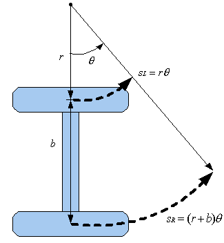
Rounding a CornerBefore tackling the differential steering model, let's consider the problem of getting a robot with a to make a 90-degree turn around a corner in a hallway or a road. A simple approach is to have the robot drive to the intersection, stop, and pivot. Clearly, though, such an approach is inefficient and a bit ungainly. A more elegant approach would be for the robot to round the corner, following a gradual circular arc through the intersection while maintaining a steady speed. To accomplish this end, we increase the speed of the outer wheel while slowing that of the inner.Is the path that the robot follows truly circular, or is it some other kind of curve? Later on, we will show that if both wheels turn at constant, but different, speeds, the robot does indeed follow a circular path. For now, just assume that path is circular. With that in mind, we see that wheel speeds are selected based on how wide a turn we desire the robot to make. |
 |
|
| Figure 1. Path of wheels through a turn. |
| Referring to Figure 1, observe the relationships: |
|
|
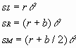
where  give the displacement (distance traveled) for the left and right wheels respectively, give the displacement (distance traveled) for the left and right wheels respectively,  is the turn radius for the inner (left) wheel, is the turn radius for the inner (left) wheel,  is the distance between wheels (from center-to-center along the length of the axle), and is the distance between wheels (from center-to-center along the length of the axle), and  is the angle of the turn in radians ( is the angle of the turn in radians ( ). ).  is the speed at the center point on the main axle. In this discussion, we will treat the axle's center point as the origin of the simulated robot's frame of reference. is the speed at the center point on the main axle. In this discussion, we will treat the axle's center point as the origin of the simulated robot's frame of reference.
Once we've established the simple geometry for the differential steering system, it is easy to develop algorithms for controlling the robot's path. Note, though, that we did make an important simplifying assumption: the wheels maintain a steady velocity. We neglected the effects of acceleration. If the wheels are allowed to accelerate, the curve which describes the robot's trajectory can become much more complicated. When working with very light robots, where the mass (and inertia) of the platform is small, we can often get away with treating changes in speed as nearly instantaneous. The path that the robot follows will not be truly circular, but it will be close enough for many applications. For larger, heavier robots, of course, mass is important and acceleration must be considered. Some Preliminaries to Developing a ModelIn the discussion above, we considered the problem of trying to choose wheel speeds based on a desired path. Now we will consider the opposite problem: how do we find the trajectory of the robot if we are told what speeds the wheels will be turning? The answer to this question leads to the development of our model and also turns out to be directly applicable to dead reckoning. Essentially, this is a problem in what is called forward kinematics, the technique of predicting a mechanical system's behavior based on the inputs to that system.Developing a model for the differential steering system is not difficult, but does require the use of calculus and differential equations. If you are unfamiliar with calculus, you may prefer to just view the results given in equations [3] and [5] below. To begin, consider that what we're really interested in is how x and y coordinates (and orientation) change with respect to time. At any instant, the x and y coordinates of the robot's center point are changing based on its speed and orientation. We treat orientation as an angle q measured in radians, counter-clockwise from the x-axis. Recall that the vector giving the direction of forward motion for the robot will be simply These observations suggest that, taking |
 . The x and y coordinates for the robot's center point will change depending on the speed of its motion along that vector.
 and
and  as time-dependent functions for the robot's speed and orientation, our solution is going to be in the form:
 , , |
[1] |
The DerivationLet's derive functions for the robot's trajectory. For now, it will be easier to defer thinking about acceleration and just assume that the speeds of the wheels are constant. If both wheels are moving at the same velocity, the robot travels in a straight line and the equation for its trajectory is trivial. So, instead, we will consider the case where the wheels travel at different velocities. |
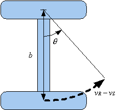 |
Referring to figure 2, note that as the robot changes position, all points on the robot may be in motion. To develop a forward kinematic equation for the motion of a differential steering system, we start by specifying a frame of reference in which an arbitarily chosen point is treated as stationary. All other points in the system are treated as moving relative to the reference point. The robot is considered a rigid body. By approaching the problem in this manner, we will gain insights which can be applied to the more general problem of modeling the robot's motion in an absolute frame of reference. | |
| Figure 2. Wheels at different velocities. |
|
The point that we select as our reference is the center point of the left wheel. This is the point where an idealized wheel makes contact with the floor. Again, all motion in this frame of reference is treated in relative to the left-wheel point. Because the right wheel is mounted perpendicular to the axle, its motion within the frame of reference follows a circular arc with a radius corresponding to the length of the axle (from hub center to hub center). Now the central point itself may be in motion, so the actual path of the right wheel will not necessarily correspond to that particular circular arc. But the change in orientation Based on these observations, we can derive a differential equation describing the change in orientation as with respect to time of time. The definition of an angle given in radians is the length of a circular arc divided by the radius of that circle. The relative velocity of the right wheel gives us that length of arc per unit time. The length from the wheel to the center point gives us the radius. Combining these facts, we have: |
 |
[2] |
|
Integrating [2] and taking the initial orientation of the robot as |
 , we find a function for calculating the robot's orientation as a function of wheel velocity and time:
 |
[3] |
|
As noted above, this change in orientation also applies to the absolute frame of reference. Shifting our attention back to the absolute frame, we recall from [1] above that the robot's overall motion depends on the the velocity its center point (the midpoint of the axle). That velocity is simply the average of that for the two wheels, or |
 . We combine this fact with what we know the about orientation as a function of time, and get the following differential equations:
  |
[4] |
|
Note that the equations in [4] are in the same form as that shown in [1]. Integrating and applying the initial position of the robot |
 , we have
  |
[5] |
|
Note that the equations given in [5] confirm the earlier assertion that, when the wheels turn at fixed velocities, the robot follows a circular path. The term When using [5] in a computer application, it is necessary to implement special handling for cases where the wheel speeds are nearly equal and Dead Reckoning and OdometryOnce we have [5], it's a small step to be able to perform dead reckoning. In traditional aviation or nautical navigation, the term "dead reckon" means to estimate position without external references. Position is dead reckoned using knowledge about a vehicle's course and speed over a period of time. In robotics, the necessary information is often obtained by measuring wheel revolutions. Devices called encoders are coupled to a robot's drive wheels and act like digital odometers. Although things can go wrong (as when the robot "spins out" on a slippery floor), encoders generally provide a good estimate of displacements for the right and left wheels, respectively. These displacement values can, in turn, be used to determine position based on odometry calculations. for the right and left wheels, respectively. These displacement values can, in turn, be used to determine position based on odometry calculations.
The equations given in [5] can be used for dead reckoning by substituting A Simpler Formula for Dead ReckoningMany popular authors on robotics recommend the formulas shown in [6] below as a way to avoid the complications that we saw in [5]. For example, Johann Borenstein, et al., propose something very similar in their widely-cited web book Where Am I? - Systems and Methods for Mobile Robot Positioning. The methods in [6] are especially well suited to small robot applications where on-board computing power is limited (and floating-point operations might not be available). |
 is actually the turn radius for circular trajectory of the robot's center.
 . In such cases, of course, the robot travels in a nearly straight line. Using L'Hospital's rule from elementary calculus, we can show that the equations do have limits approaching a straight line in the direction of the initial orientation
  .
. and dropping the time value
  , then solving for the values
  , and
, and 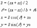 |
[6] |
|
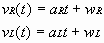
The forumulas in [6] are simple and convenient. They work well for algorithms as long as you remember that they are approximations... a fact that is sometimes overlooked. Essentially, [6] computes the robot's total rotation and distance traveled, then treats it as if it had completed the full rotation as a pivot the very beginning of the maneuver and then traveled in a straight line. Of course, this kind of "point-and-shoot" description is an incomplete representation of the reality. But so long as the robot's actual path doesn't involve too much of a turn, everything is fine. How much of a turn is too much? That depends on the geometry of the particular robot. You can probably use [6] as long as the angle of the turn does not get larger than 10 degrees. If it does, you should apply the approximation in stages. That is, if the robot's transit results in a turn of 20 degrees, treat it as two segments of 10 degrees each. Updated June 2004: Tom Brown of the University of Illinois at Urbana-Champaign proposes a nice little improvement to [6]. Imagine that the robot is following a circular path curving to the left. It is easy to see that the point-and-shoot maneuver described above would create a path to the inside of the curve. Tom suggests that the accuracy of the approximation can be improved by simply dividing the robot's change in orientation by two. So the theta term in the equations becomes Whether you apply [5] or [6] for your dead reckoning, remember that the realities of mechanical systems limit the accuracy of your calculations. If the robot's wheels hit a slippery spot on the floor and spin wildly, it will degrade the accuracy of the distances measured by the encoders. Even when your wheels maintain traction, your position estimates will be vulnerable to backlash (slop) in the robot's gearing, inaccuracies in the encoders, and small variations in the wheel speed. AccelerationAdding acceleration to the model is simply a matter of substituting appropriate time-dependent equations for wheel velocities into [2] and [4]. Unfortunately, the resulting differential equations are often not solvable, but must be evaluated using numerical methods. Let's consider a simple example where the wheels undergo a fixed rate of acceleration. Let |
 . When adjusted this way, the point-and-shoot path will not be so far inside the curved path and, eventually, the two may even cross. Tom also generously provided an upgrade to the
  |
[7] |
|
give the velocities of the right and left wheels where |
 give the values for a constant acceleration (or deceleration) and
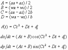
  give the initial velocities. Substituting into [2] and [4] we have
 |
[8] |
|
We were able to solve the differential equation for orientation directly. The equations for position are intractable and must be evaluated numerically. Jing YE, a student at the University of Melbourne, recently used Simpson's Rule, a technique from elementary calculus, to add a treatment of acceleration to Michael Gauland's MotionApplet. In the real world, when a robot applies constant power to a wheel, it does not achieve a constant rate of acceleration. As the parts of the drive system turns faster, it experiences greater internal friction and requires more and more power to realize the same increase in speed. Based on your own system characteristics, you may wish to implement an acceleration model based on a time-dependent polynomial rather than the linear function used in [7]. An even more sophisticated analysis might yield better, more complicated functions for velocity and acceleration. Due to the inaccuracies inherent in robot mechanical systems, however, you will soon reach a point where improving the model is worth neither the human effort or extra CPU processing power needed to do so. |
Direct comments to: gwlucas@users.sourceforge.net.
로봇 휠 액츄에이터의
차동 조향 시스템에 대한 튜토리얼 및 기본 궤적 모델
작성자: GW 루카스
내용물
Rossum 프로젝트 자원봉사자 중 한 명인 Michael Gauland는 최근
이 문서의 개념을 설명하는 깔끔하고 작은 Java 애플릿을 기고했습니다. 애플릿을 보려면 [여기]를 클릭하세요.


소개이 노트는 차동 조종 드라이브 시스템 이 장착된 로봇이나 차량의 경로를 설명하는 방정식을 제시합니다 . 이 간단하고 안정적인 바퀴 기반 추진 시스템은 일반적으로 소형 로봇에 사용됩니다. 이는 본질적으로 휠체어에 사용되는 시스템과 동일하기 때문에 일상 생활에 익숙합니다. 단일 축에 장착된 두 개의 바퀴가 독립적으로 구동 및 제어되어 구동 및 조향 기능을 모두 제공합니다. 이 노트의 방정식은 차동 조향 구동 시스템(종종 차동 조향 시스템이라고 함)에 대한 기본 모델을 제공합니다. 이 모델은 이러한 시스템을 갖춘 로봇이 휠 속도 변화에 어떻게 반응하는지, 다양한 조건에서 로봇이 어떤 경로를 따라갈지 예측하는 데 사용할 수 있습니다. 이 모델은 또한 주행 거리 측정 애플리케이션(각 바퀴에 장착된 주행 거리계 장치로 측정된 거리를 기반으로 로봇의 위치를 추정하는 기술)을 통해 추측 항법 또는 위치 파악에서 로봇의 위치를 계산하는 데 사용할 수 있습니다 .여기에 제공된 방정식은 로봇이나 차량의 동작에 대한 기본 모델을 나타낸다는 점을 강조할 가치가 있습니다 . 그들은 로봇의 위치와 방향을 바퀴 움직임의 함수로 설명하지만 해당 움직임을 발생시키는 데 관련된 기본 물리학을 무시합니다. 토크와 힘, 마찰, 에너지, 관성과 같은 문제는 좀 더 심화된 논의를 위해 남겨두겠습니다. 기술적인 용어로 이러한 동작을 설명하는 방법을 운동학 접근 방식 이라고 합니다 . 이는 운동의 원인( 역학 접근 방식 에서 연구됨 )을 무시하고 효과에 중점을 둡니다. 또한 이 노트에서는 휠 기반 액추에이터를 가능하게 하는 모터, 기어링, 전자기학, 전원 공급 장치 및 기타 엔지니어링 고려 사항에 대한 많은 흥미로운 세부 사항을 무시합니다. 따라서 이는 완전한 설명이 아니라 차등적으로 조종되는 구동 시스템을 갖춘 로봇의 동작을 이해하는 첫 번째 단계를 제공합니다. 이 웹 페이지의 대상 독자에는 차동 조향 모델을 개발하는 데 사용되는 미적분 기술에 익숙하지 않은 고등학생 및 학부생이 포함됩니다. 이러한 학생들은 텍스트를 살펴보고 방정식 [3] 및 [5]의 결과에 주의를 기울여 관련 정보를 "분석"할 수 있어야 합니다. 모델을 실제로 활용하려면 모델 뒤에 숨은 수학과 운동학에 대한 이해가 필요합니다. 따라서 이 페이지의 토론에는 문제에 대한 많은 배경 정보와 관례적인 설명보다 더 많은 양의 설명이 포함됩니다. 많은 세부 정보를 제공함으로써 이 노트는 독자가 차동 조향 모델을 자신의 로봇 응용 프로그램에 적용하는 데 도움이 될 것입니다. 차동 조향 시스템은 때때로 "차동 구동 시스템"으로 잘못 불립니다. 차동 구동이라는 용어는 자동차 엔지니어링에서 차동 기어 또는 관련 장치(전통적인 후륜 구동 차량에서와 같이)를 통해 구동 휠에 동력을 전달하는 일종의 추진 시스템을 나타내는 데 사용됩니다. 분명히 여기에 설명된 시스템과는 다른 개념입니다. 로봇 공학 애호가들은 구별하는 데 주의를 기울입니다. 마지막으로, 모델에 사용된 접근 방식을 제안한 재능 있는 수학자이자 엔지니어인 Albert Gerheim의 공헌에 감사의 말씀을 전하고 싶습니다. 차동 조향 시스템위에서 언급했듯이 많은 로봇에 사용되는 차동 조향 구동 시스템은 본질적으로 휠체어에 사용되는 것과 동일한 배열입니다. 따라서 우리 대부분은 그것이 행동하는 방식을 직관적으로 파악하고 있습니다. 두 구동바퀴가 동시에 회전하면 로봇은 직선으로 움직입니다. 한 바퀴가 다른 바퀴보다 빠르게 회전하면 로봇은 느린 바퀴를 향해 안쪽으로 곡선 경로를 따라갑니다. 바퀴가 동일한 속도로 회전하지만 반대 방향으로 회전하면 로봇이 회전합니다. 따라서 로봇을 조종하는 것은 단지 구동 휠의 속도를 변화시키는 문제일 뿐입니다. 하지만 로봇이 원하는 곳으로 이동하려면 속도를 정확히 어떻게 선택해야 할까요? 이 노트에서는 이러한 직관적인 이해를 로봇 제어 소프트웨어 구현에 사용할 수 있는 수학적 표현으로 구체화하려고 노력할 것입니다. |
코너 라운딩차동 조향 모델을 다루기 전에 로봇이 복도나 도로의 모퉁이를 90도 회전하는 문제를 고려해 보겠습니다. 간단한 접근 방식은 로봇이 교차로까지 주행하고 정지한 후 회전하도록 하는 것입니다. 하지만 분명히 그러한 접근 방식은 비효율적이며 다소 보기 흉합니다. 보다 우아한 접근 방식은 로봇이 일정한 속도를 유지하면서 교차점을 통과하는 점진적인 원호를 따라 모퉁이를 둥글게 돌아가는 것입니다 . 이 목적을 달성하기 위해 우리는 바깥쪽 바퀴의 속도를 높이고 안쪽 바퀴의 속도를 늦춥니다.로봇이 따라가는 경로는 진정한 원형인가요, 아니면 다른 종류의 곡선인가요? 나중에 두 바퀴가 일정하지만 다른 속도로 회전하는 경우 로봇이 실제로 원형 경로를 따른다는 것을 보여줄 것입니다. 지금은 경로가 원형이라고 가정합니다. 이를 염두에 두고 로봇이 원하는 회전 폭에 따라 휠 속도가 선택된다는 것을 알 수 있습니다. |
|
|
| 그림 1. 회전을 통한 바퀴의 경로. |
| 그림 1을 참조하여 관계를 살펴보세요. |
|
|
| 여기서 각각 왼쪽 및 오른쪽 바퀴의 변위(이동 거리) 는 내부(왼쪽) 바퀴의 회전 반경이고, 는 바퀴 사이의 거리(축 길이를 따라 중심에서 중심까지)이며 , 회전 각도(라디안)( ). 는 주축 중심점에서의 속도입니다. 이 논의에서는 축의 중심점을 시뮬레이션된 로봇의 기준 프레임의 원점으로 처리합니다.
차동 조향 시스템을 위한 간단한 형상을 확립하고 나면 로봇의 경로를 제어하기 위한 알고리즘을 쉽게 개발할 수 있습니다. 그러나 우리는 중요한 단순화 가정을 세웠다는 점에 유의하십시오: 바퀴는 일정한 속도를 유지합니다. 우리는 가속의 효과를 무시했습니다. 바퀴의 가속이 허용되면 로봇의 궤적을 나타내는 곡선이 훨씬 더 복잡해질 수 있습니다. 플랫폼의 질량(및 관성)이 작은 매우 가벼운 로봇으로 작업할 때 속도 변화를 거의 순간적으로 처리할 수 있는 경우가 많습니다. 로봇이 따르는 경로는 진정한 원형은 아니지만 많은 응용 분야에 충분히 가깝습니다. 더 크고 무거운 로봇의 경우 당연히 질량이 중요하고 가속도도 고려해야 합니다. 모델 개발을 위한 몇 가지 준비 사항위의 논의에서 우리는 원하는 경로를 기반으로 휠 속도를 선택 하려는 문제를 고려했습니다 . 이제 우리는 반대 문제를 고려해 보겠습니다. 바퀴가 어떤 속도로 회전할지 알 수 있다면 로봇의 궤적을 어떻게 찾을 수 있습니까 ? 이 질문에 대한 답은 우리 모델의 개발로 이어졌고 추측항법에도 직접 적용할 수 있는 것으로 나타났습니다. 본질적으로 이는 해당 시스템에 대한 입력을 기반으로 기계 시스템의 동작을 예측하는 기술인 순운동학 이라는 문제입니다 .차동 조향 시스템용 모델을 개발하는 것은 어렵지 않지만 미적분학 및 미분 방정식을 사용해야 합니다. 미적분학에 익숙하지 않은 경우 아래 방정식 [3] 및 [5]에 제공된 결과를 보는 것이 더 나을 수 있습니다. 시작하려면, 우리가 실제로 관심을 갖는 것은 시간에 따라 x와 y 좌표(및 방향)가 어떻게 변하는가입니다. 어떤 순간에도 로봇 중심점의 x 및 y 좌표는 속도와 방향에 따라 변경됩니다. 방향을 x축에서 시계 반대 방향으로 라디안 단위로 측정된 각도 q 로 처리합니다. 로봇의 전진 동작 방향을 지정하는 벡터는 간단하다는 점을 기억하세요 이러한 관찰은 로봇의 속도와 방향에 대한 시간 의존 함수로서 우리의 솔루션이 다음과 같은 형식이 될 것임을 시사 |
| , |
[1] |
파생로봇의 궤적에 대한 함수를 도출해 보겠습니다. 지금은 가속에 대한 생각을 미루고 바퀴의 속도가 일정하다고 가정하는 것이 더 쉬울 것입니다. 두 바퀴가 동일한 속도로 움직이는 경우 로봇은 직선으로 이동하며 궤적에 대한 방정식은 간단합니다. 그래서 대신에 바퀴가 다른 속도로 움직이는 경우를 고려해 보겠습니다. |
|
그림 2를 참조하면 로봇의 위치가 변경됨에 따라 로봇의 모든 지점이 움직일 수 있습니다. 차동 조향 시스템의 운동에 대한 순운동학 방정식을 개발하기 위해 임의로 선택한 점이 고정된 것으로 간주되는 기준 프레임을 지정하는 것부터 시작합니다. 시스템의 다른 모든 점은 참조점을 기준으로 이동하는 것으로 간주됩니다. 로봇은 강체로 간주됩니다. 이러한 방식으로 문제에 접근함으로써 우리는 절대 기준계에서 로봇의 동작을 모델링하는 보다 일반적인 문제에 적용할 수 있는 통찰력을 얻을 수 있습니다. | |
| 그림 2. 다양한 속도의 바퀴. |
|
기준으로 선택한 점은 왼쪽 바퀴의 중심점입니다. 이것은 이상적인 바퀴가 바닥과 접촉하는 지점입니다. 다시 말하지만, 이 기준 프레임의 모든 동작은 왼쪽 바퀴 지점을 기준으로 처리됩니다. 오른쪽 바퀴는 축에 수직으로 장착되어 있기 때문에 기준 프레임 내에서 의 움직임 은 축의 길이(허브 중심에서 허브 중심까지)에 해당하는 반경을 갖는 원호를 따릅니다. 이제 중심점 자체가 움직일 수 있으므로 오른쪽 바퀴의 실제 경로가 반드시 특정 원호와 일치하지는 않습니다. 그러나 방향 변화는 로봇의 기준 틀에만 국한되지 이러한 관찰을 바탕으로 시간에 따른 방향 변화를 설명하는 미분 방정식을 유도할 수 있습니다. 라디안으로 주어진 각도의 정의는 원호의 길이를 해당 원의 반지름으로 나눈 값입니다. 오른쪽 바퀴의 상대 속도는 단위 시간당 호의 길이를 제공합니다. 바퀴에서 중심점까지의 길이가 반경을 제공합니다. 이러한 사실을 종합하면 다음과 같습니다. |
|
[2] |
|
[2]를 적분하고 로봇의 초기 방향을 로 취하면 |
|
[삼] |
|
위에서 언급한 바와 같이 이러한 방향 변경은 절대 기준계에도 적용됩니다. 절대 프레임으로 다시 관심을 돌리면 위의 [1]에서 로봇의 전체 동작이 중심점(축의 중간점) 속도에 따라 달라진다는 점을 상기해 보겠습니다. 그 속도는 단순히 두 바퀴의 평균, 즉 |
|
[4] |
|
[4]의 방정식은 [1]에 표시된 것과 동일한 형식입니다. 로봇의 초기 위치를 적분하고 적용하면 |
|
[5] |
|
[5]에 주어진 방정식은 바퀴가 고정된 속도로 회전할 때 로봇이 원형 경로를 따른다는 이전 주장을 확인합니다. 이 용어는 컴퓨터 애플리케이션에서 [5]를 사용할 때 휠 속도가 거의 같고 추측 항법 및 주행 거리 측정[5]가 있으면 추측 항법을 수행할 수 있는 작은 단계입니다. 전통적인 항공 또는 해상 항법에서 " 추측 항법 "이라는 용어는 외부 참조 없이 위치를 추정하는 것을 의미합니다. 위치는 일정 기간 동안 차량의 경로와 속도에 대한 지식을 사용하여 추정됩니다. 로봇 공학에서는 휠 회전을 측정하여 필요한 정보를 얻는 경우가 많습니다. 인코더라고 불리는 장치는 로봇의 구동 휠에 연결되어 디지털 주행 거리계처럼 작동합니다. 로봇이 미끄러운 바닥에서 "회전"할 때와 같이 상황이 잘못될 수 있지만 일반적으로 인코더는 각각 오른쪽 및 왼쪽 바퀴의 변위에 대한 좋은 추정치를 제공합니다. 이러한 변위 값은 주행 거리 계산을 기반으로 위치를 결정하는 데 사용될 수 있습니다.
추측 항법을 위한 더 간단한 공식로봇 공학 분야의 많은 유명 저자들은 [5]에서 본 복잡성을 피하는 방법으로 아래 [6]에 표시된 공식을 권장합니다. 예를 들어, Johann Borenstein 등은 널리 인용되는 웹 서적 Where Am I? 에서 매우 유사한 것을 제안했습니다. - 모바일 로봇 포지셔닝을 위한 시스템 및 방법 . [6]의 방법은 온보드 컴퓨팅 성능이 제한되어 있는(부동 소수점 연산을 사용할 수 없는) 소형 로봇 애플리케이션에 특히 적합합니다. |
|
[6] |
|
[6]의 공식은 간단하고 편리합니다. 근사치라는 점을 기억하는 한 알고리즘에 잘 작동합니다. 이는 때때로 간과되는 사실입니다. 기본적으로 [6]은 로봇의 전체 회전과 이동 거리를 계산한 다음 로봇이 기동 초기에 피벗으로 전체 회전을 완료한 다음 직선으로 이동한 것처럼 처리합니다. 물론 이런 종류의 '조준식' 설명은 현실을 불완전하게 표현한 것입니다. 그러나 로봇의 실제 경로가 너무 많은 회전을 포함하지 않는 한 모든 것이 정상입니다. 얼마나 많은 회전이 너무 큽니까 ? 이는 특정 로봇의 기하학적 구조에 따라 다릅니다. 회전 각도가 10도를 초과하지 않는 한 [6]을 사용할 수 있습니다. 그렇다면 단계적으로 근사치를 적용해야 합니다. 즉, 로봇의 이동으로 인해 20도 회전하는 경우 이를 각각 10도씩 두 개의 세그먼트로 처리합니다. 2004년 6월 업데이트: 일리노이 대학교 Urbana-Champaign의 Tom Brown은 [6]에 대한 약간의 개선을 제안했습니다. 로봇이 왼쪽으로 휘어지는 원형 경로를 따라가고 있다고 상상해 보세요. 위에서 설명한 조준 사격 조작이 곡선 내부로 가는 경로를 생성한다는 것을 쉽게 알 수 있습니다. Tom은 단순히 로봇의 방향 변화를 2로 나누면 근사치의 정확도가 향상될 수 있다고 제안합니다. 따라서 방정식의 세타 항은 가 됩니다 추측항법에 [5]를 적용하든 [6]을 적용하든 기계 시스템의 현실은 계산의 정확성을 제한한다는 점을 기억하십시오. 로봇의 바퀴가 바닥의 미끄러운 부분에 부딪혀 격렬하게 회전하면 인코더가 측정한 거리의 정확도가 저하됩니다. 바퀴가 견인력을 유지하더라도 위치 추정은 로봇 기어링의 백래시(경사), 인코더의 부정확성 및 바퀴 속도의 작은 변화에 취약합니다. 가속모델에 가속도를 추가하는 것은 단순히 바퀴 속도에 대한 적절한 시간 종속 방정식을 [2]와 [4]에 대체하는 문제입니다. 불행하게도 결과로 나온 미분 방정식은 풀 수 없는 경우가 많으므로 수치적 방법을 사용하여 평가해야 합니다. 바퀴가 고정된 가속도를 받는 간단한 예를 생각해 보겠습니다. 허락하다 |
|
[7] |
|
|
|
[8] |
|
우리는 방향에 대한 미분 방정식을 직접 풀 수 있었습니다. 위치에 대한 방정식은 다루기 어렵고 수치적으로 평가해야 합니다. 멜버른 대학의 학생 Jing YE는 최근 초등 미적분학의 기술인 Simpson's Rule을 사용하여 Michael Gauland의 MotionApplet에 가속 처리 기능을 추가 했습니다 . 현실 세계에서는 로봇이 바퀴에 일정한 힘을 가할 때 일정한 가속도를 달성하지 못합니다. 구동 시스템의 부품이 더 빠르게 회전함에 따라 내부 마찰이 더 커지며 동일한 속도 증가를 실현하려면 점점 더 많은 전력이 필요합니다. 자신의 시스템 특성에 따라 [7]에서 사용된 선형 함수 대신 시간 종속 다항식을 기반으로 한 가속 모델을 구현하고 싶을 수도 있습니다. 더욱 정교한 분석을 통해 속도와 가속도에 대한 더 좋고 복잡한 함수를 얻을 수 있습니다. 그러나 로봇 기계 시스템에 내재된 부정확성으로 인해 모델을 개선하는 데 필요한 인간의 노력이나 추가 CPU 처리 능력이 가치가 없는 지점에 곧 도달하게 될 것입니다. |
의견은 gwlucas@users.sourceforge.net으로 보내주세요 .
[출처] https://rossum.sourceforge.net/papers/DiffSteer/
광고 클릭에서 발생하는 수익금은 모두 웹사이트 서버의 유지 및 관리, 그리고 기술 콘텐츠 향상을 위해 쓰여집니다.
